import os
import numpy as np
import matplotlib.pyplot as plt

DATA = "data"
plt.rcParams.update({"figure.dpi": 130, "font.size": 10, "axes.grid": True,
                     "grid.alpha": 0.3, "axes.axisbelow": True,
                     "figure.facecolor": "white", "savefig.bbox": "tight"})
C_PECLET, C_TBF, C_TBFNS = "#2a78d6", "#e34948", "#f0a04b"


def ld(name):
    p = os.path.join(DATA, name + ".npz")
    return np.load(p, allow_pickle=True) if os.path.exists(p) else None


pec, tbf, tbfns = ld("peclet_closed"), ld("tbf_closed_t150"), ld("tbf_closed_nosmooth_t150")
RUNS = ((pec, C_PECLET, "peclet.flow"), (tbf, C_TBF, "TBFsolver"),
        (tbfns, C_TBFNS, "TBFsolver, no smoothing"))
T0, T1 = 50.0, 150.0


def first(a):                       # TBFsolver stores 3-vectors, peclet the vertical component
    a = np.asarray(a)
return a[:, 0] if a.ndim == 2 else aA bubble column, run twice: peclet.flow vs TBFsolver
Sixteen deformable bubbles rising in a closed column between two walls, on the same grid from the same initial state, in peclet’s multiple-marker VoF and in TBFsolver — the reference implementation of that method — with an isolated-bubble, a drafting-pair and a published-swarm check to say where they agree and where they do not.
flow
VoF
bubbly flow
accuracy
performance
benchmark
validation
What this measures
A bubble column is the simplest bubbly flow with a large-scale structure of its own: gas rises, the liquid it displaces has to come back down, and in a closed column it does so along the walls. This page runs one such column with two codes that implement the same method:
- TBFsolver (Cifani et al., “Highly scalable DNS solver for turbulent bubble-laden channel flow”, Computers & Fluids 2018) — the MPI+OpenMP Fortran code that introduced multiple-marker VoF on moving blocks: every bubble carries its own volume-fraction field on its own small box, so two bubbles that touch can never merge numerically.
peclet.flow— the same container (one Weymouth–Yue geometric VoF field per bubble on a moving box, the union colour \(\max_k C_k\) for density and viscosity, each bubble’s own balanced-force surface tension summed into the momentum equation) on Kokkos.
Both runs use the same 128 × 96 × 64 cubic grid, the same 16 bubble centres, the same physical parameters and the same closed-column forcing, so every difference below is a difference of discretisation, not of set-up.
NoteWhat building this benchmark found and fixed in peclet
Three defects, none of which the regression suite could see:
- Colliding bubbles blew up — garbage curvature on sub-cell debris one marker leaves inside another (below).
- A bubble touching the lower wall leaked volume (up to 3 % per bubble within 40 time units): the per-bubble advection read a non-zero velocity on the lower domain face, where the wall has none.
- Bubbles collected at the lower wall — in the case and in its mirror image. The variable viscosity sat half a cell off the staggered control volume, which made the viscous term first order and, in the wall-normal direction, asymmetric. A mirror-symmetry test now guards it.
Every result on this page is from the corrected code (peclet.flow main, 2026-09-25 onwards).
The case
Units: bubble diameter \(D\), liquid density \(\rho_l\) and gravity \(g\) are 1. The bubbles are case E1 of Loisy, Naso & Spelt (J. Fluid Mech. 816, 2017) — Archimedes number \(Ar = \sqrt{\rho_l(\rho_l-\rho_g) g D^3}/\mu_l = 29.9\) and Bond number \(Bo = (\rho_l-\rho_g) g D^2/\sigma = 2.0\), weakly ellipsoidal bubbles whose isolated rise Reynolds number is about 31 (Loth 2008) — with density and viscosity ratios \(\rho_g/\rho_l = \mu_g/\mu_l = 0.02\) as in Bunner & Tryggvason (J. Fluid Mech. 466, 2002).
| column | \(8D\) tall (periodic), \(6D\) between the no-slip walls, \(4D\) deep (periodic) |
| grid | 128 × 96 × 64 cubic cells, \(D/h = 16\) (checks at 24) |
| bubbles | 16, a perturbed 4 × 2 × 2 array; void fraction 4.36 % |
| forcing | \((\rho - \langle\rho\rangle)\,g\) along the column, and zero net volume flux |
| run | \(t = 0 \ldots 150\,\sqrt{D/g}\); statistics over \(t \in [50, 150]\) |
| pressure | exact variable-coefficient projection, MG-PCG to relative residual \(10^{-8}\) |
The zero-net-flux constraint makes this a batch column: without it, the liquid descending along the walls feels an upward wall friction that nothing balances, and the whole column develops a growing net upflow. Both codes remove the mean volume flux every step (TBFsolver flowCtrl 2, peclet set_superficial_velocity(True, "x", 0.0)).
TBFsolver by default smooths density and viscosity across the interface; peclet does not. We ran TBFsolver both ways.
Rise speed
The observable is the drift velocity — the gas-phase mean velocity relative to the volume-averaged mixture velocity, positive upward — computed identically from both codes’ fields.
fig, ax = plt.subplots(figsize=(6.5, 3.2))
ax.axvspan(T0, T1, color="0.93", zorder=0)
for z, c, lab in RUNS:
    ax.plot(z["t"], z["rise_speed"], color=c, lw=1.1, label=lab)
ax.set_xlabel(r"$t\,\sqrt{g/D}$")
ax.set_ylabel(r"drift velocity $/\sqrt{gD}$")
ax.legend(loc="lower right")
plt.show()

for z, c, lab in RUNS:
    m = (z["t"] >= T0) & (z["t"] <= T1)
    a, ul = z["alpha_y"][m], z["u_liq_y"][m]
    slip = -(first(z["u_gas"][m]) - (a * ul).sum(1) / a.sum(1))
    w = z["rise_speed"][m]
    print(f"{lab:24s} drift {w.mean():.3f} +- {w.std():.3f}   slip relative to the "
          f"liquid around the gas {slip.mean():.3f}")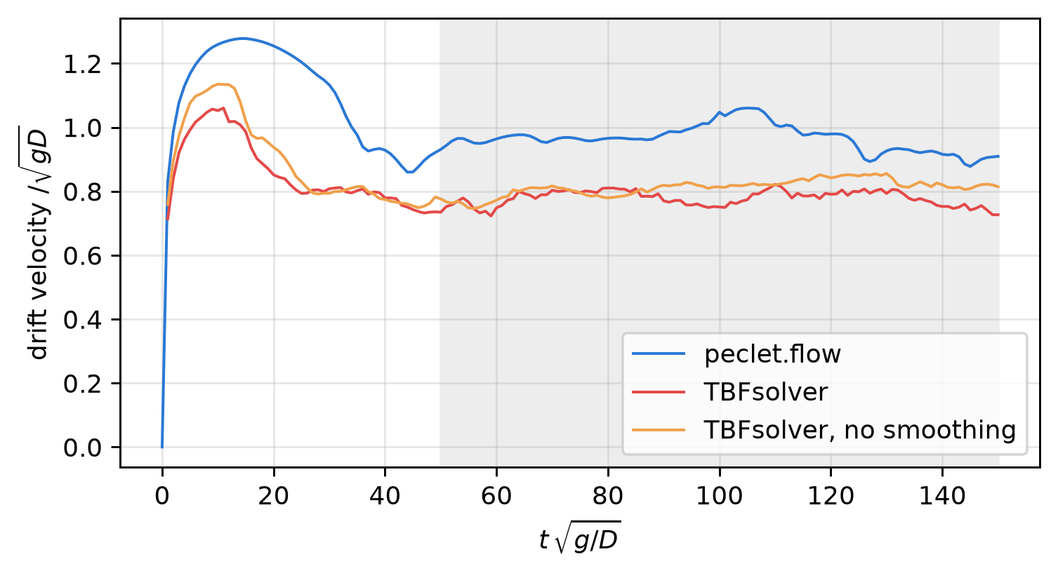
peclet.flow              drift 0.965 +- 0.042   slip relative to the liquid around the gas 0.918
TBFsolver                drift 0.778 +- 0.024   slip relative to the liquid around the gas 0.780
TBFsolver, no smoothing  drift 0.811 +- 0.025   slip relative to the liquid around the gas 0.804
peclet’s bubbles rise about 19 % faster than TBFsolver’s without smoothing (and 24 % faster than with it). The large-scale circulation is not the reason: measured against the liquid that actually surrounds the gas, the slip still differs by 14 %. Why they differ is the subject of Where the two codes differ.
The column’s structure
fig, axs = plt.subplots(1, 2, figsize=(7.5, 3.2))
for z, c, lab in RUNS:
    m = (z["t"] >= T0) & (z["t"] <= T1)
    axs[0].plot(z["y"], z["alpha_y"][m].mean(axis=0), color=c, label=lab)
    axs[1].plot(z["y"], z["u_liq_y"][m].mean(axis=0), color=c, label=lab)
axs[0].set_xlabel("$y/D$"); axs[0].set_ylabel(r"void fraction $\langle\alpha\rangle$")
axs[1].set_xlabel("$y/D$"); axs[1].set_ylabel(r"liquid velocity $/\sqrt{gD}$")
axs[0].legend(fontsize=8)
plt.tight_layout(); plt.show()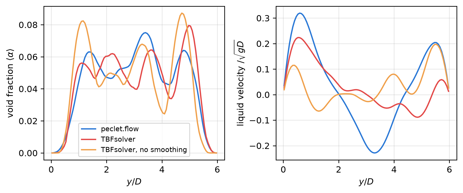
Both codes put the gas in the core (void fraction ≈ 0.053 in the middle, ≈ 0.01 near the walls) with the liquid coming down along both walls.
Conservation
fig, ax = plt.subplots(figsize=(6.5, 3.0))
for z, c, lab in RUNS:
    v = z["marker_volume_total"] if "marker_volume_total" in z else z["gas_volume"]
    ax.plot(z["t"], v / v[0] - 1, color=c, label=lab)
ax.set_xlabel(r"$t\,\sqrt{g/D}$"); ax.set_ylabel("relative gas volume change")
ax.legend(); plt.show()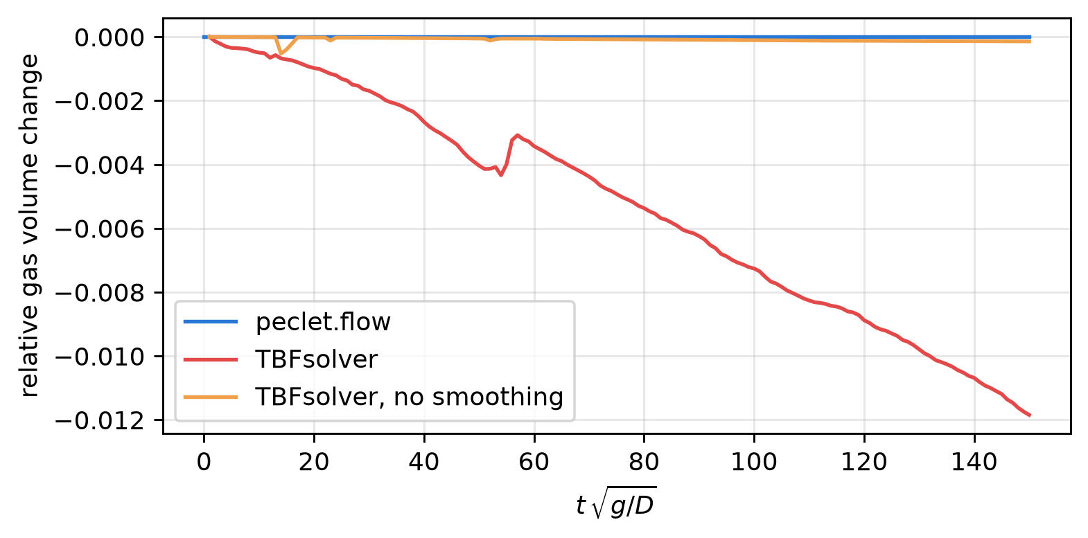
peclet: \(+1.3\times10^{-10}\) after 94 980 steps (\(-7\times10^{-13}\) with the pressure solved to \(10^{-10}\); the case runs at \(10^{-8}\), which needs 24 % fewer pressure iterations). TBFsolver: \(-1.2\,\%\) (with smoothing), \(-1.4\times10^{-4}\) (without).
Where the two codes differ, and why
The column mixes everything — single-bubble drag, wake interaction, near-contact — so we separated them.
One bubble. In the same walled box, peclet and TBFsolver without smoothing agree within 1–4 %; TBFsolver’s smoothing slows a lone bubble by 8–14 %:
| terminal rise speed | peclet | TBFsolver, no smoothing | TBFsolver |
|---|---|---|---|
| box 4 × 4 × 4 \(D\) (periodic image 4 \(D\) above) | 1.300 | 1.309 | 1.155 |
| box 8 × 4 × 4 \(D\) | 1.077 | 1.122 | 0.989 |
| box 2 × 4 × 4 \(D\) (in its own wake at the column’s spacing) | 1.770 | 1.746 | 1.522 |
Two bubbles. A trailing bubble released 2 \(D\) below a leading one, offset sideways by \(0.1D\): before contact the lateral dynamics are the same in both codes. They part at near contact — and both do something set by the grid, not by physics:
| drafting pair | closest film (centre–centre) | trailing bubble passes at |
|---|---|---|
| peclet, \(D/h = 16\) | \(+0.163D\) = 2.6 cells (0.93 \(D\)) | \(t = 20.6\) |
| peclet, \(D/h = 24\) | \(+0.066D\) = 1.6 cells (0.86 \(D\)) | \(t = 18.1\) |
| TBFsolver (no smoothing), \(D/h = 16\) | \(-0.051D\), overlap 0.8 cells (0.74 \(D\)) | \(t = 12.1\) |
| TBFsolver (no smoothing), \(D/h = 24\) | \(-0.033D\), overlap 0.8 cells (0.74 \(D\)) | \(t = 13.1\) |
peclet keeps a liquid film of a couple of cells that resists draining, so the pair “tumbles” slowly; TBFsolver lets the two markers interpenetrate by about one cell and passes quickly. peclet’s film thins faster than the grid spacing, so it is not converged lubrication either; the two codes move towards each other with refinement. Neither resolves real film drainage at these grids (the single-field VoF path in peclet reproduces the multiple-marker pair to \(10^{-5}D\), so this is the flow solver’s near-contact behaviour, not the bubble container).
Many bubbles. In a swarm these near-contact encounters are where the codes part, which is why the column’s drift differs while the single-bubble and in-line-wake cases agree. Resolution does not close it: the start-up transient is converged in both codes, and peclet is 7–10 % faster from \(t = 2\) on.
rows = [("peclet.flow, D/h = 16", pec), ("peclet.flow, D/h = 24", ld("peclet_closed_d24_t60")),
        ("TBFsolver no smoothing, D/h = 16", tbfns),
        ("TBFsolver no smoothing, D/h = 24", ld("tbf_closed_nosmooth_d24_t60")),
        ("TBFsolver, D/h = 16", tbf), ("TBFsolver, D/h = 24", ld("tbf_closed_d24_t5"))]
print(f"{'':34s}" + "".join(f"   t = {k}" for k in range(1, 6)))
for lab, z in rows:
    if z is None:
        continue
    vals = [z["rise_speed"][np.argmin(abs(z["t"] - k))] for k in range(1, 6)]
    print(f"{lab:34s}" + "".join(f"   {v:.3f}" for v in vals))
t = 1 t = 2 t = 3 t = 4 t = 5
peclet.flow, D/h = 16 0.830 0.986 1.076 1.129 1.168
peclet.flow, D/h = 24 0.837 0.991 1.083 1.138 1.179
TBFsolver no smoothing, D/h = 16 0.759 0.895 0.972 1.029 1.076
TBFsolver no smoothing, D/h = 24 0.756 0.896 0.968 1.016 1.057
TBFsolver, D/h = 16 0.713 0.840 0.920 0.963 0.992
TBFsolver, D/h = 24 0.724 0.863 0.928 0.971 1.000An independent reference. Loisy, Naso & Spelt computed free swarms of exactly these E1 bubbles with a level-set method (one field; bubbles never touch at this void fraction). Eight bubbles in a triply periodic cube at void fraction 3.8 %, drift normalised by the isolated rise speed \(U_0\) (Loth):
| free array, E1, 8 bubbles, \(\phi = 3.8\,\%\) | \(U/U_0\) |
|---|---|
| peclet, multiple-marker, ratios 0.02 / 0.02 | 0.99 |
| peclet, single field, ratios 0.02 / 0.02 | 0.99 |
| peclet, single field, Loisy’s ratios (\(\rho_g/\rho_l = 10^{-3}\), \(\mu_g/\mu_l = 10^{-2}\)) | 0.89 |
| Loisy, Naso & Spelt 2017, fig. 21 | ≈ 0.80 |
The property ratios matter (0.99 → 0.89); at matching ratios peclet is about 11 % above the level-set result — the same order as the code-to-code spread from near-contact treatment above.
Reading. For a single bubble and for in-line wake interaction the two codes agree to a few per cent. In a swarm the mean rise speed is sensitive, at the 10–15 % level, to how bubbles behave at near contact — a film of one or two grid cells in peclet, an overlap of about one cell in TBFsolver, merging within a cell in a level-set code — and none of these is converged physics at \(D/h = 16\)–24. A swarm drift from any of these methods carries that uncertainty.
The collision fix
When two markers overlap, the Weymouth–Yue advection of each one leaves sub-cell debris in cells the other bubble fills: volume fractions of order \(10^{-8}\) to \(10^{-3}\) along the rim of the contact lens. Each such cell passes the “is this interfacial?” test, so the height-function cascade gives it a curvature — garbage, since nothing in its stencil is a real interface: 273 and −428 per cell were measured where the bubble’s own curvature is about 0.4 per cell. Multiplied by \(\sigma\nabla C_k\), that produced a one-step velocity blow-up. The balanced-force pairing of the per-marker forces with the union colour, which had been blamed, is exact for a constant curvature and was not the cause.
The fix, all inside the block container:
- Debris removal with exact return. After every advection, a marker’s cells that are interfacial but have no cell above \(C = \tfrac12\) within two cells are cleared, and their volume goes back to the same marker’s genuine interface, weighted by \(C(1-C)\); values below the wisp threshold (\(10^{-8}\)) likewise. Every marker’s volume is conserved to round-off.
- A curvature bound \(|\kappa| \le 1/\Delta_{\min}\) per cell on the block path, as a backstop.
- A capillary time-step bound for the gas–gas contact while markers overlap.
A two-bubble shear collision that blew up at step 2910 now completes; the bubbly channel that died at step 10 706 runs on with volumes conserved to \(2\times10^{-14}\); MPI runs at 1, 2 and 4 ranks are bitwise identical. Design and gates: doc/vof_overlap_design.md.
Cost
Measured on Snellius genoa nodes (2 × AMD EPYC 9654). TBFsolver ran on the same node in every job, both codes pinned to the same cores; peclet.flow main as of 2026-10-03 (commit d02d3b0):
| ms per step | TBFsolver | peclet.flow | peclet.flow, -march=znver4 |
|---|---|---|---|
| 24 cores (8 MPI × 3 threads) | 45–46 | 166–169 | 163 |
| 24 cores (1 × 24 threads) | — | 144 | 140 |
| 192 cores | 25 | 82–85 | 84 |
| one GPU (RTX 5080) | — | 36–37 | — |
Time steps are equal (≈ 1.55 × 10⁻³ in both), so cost per step is cost per simulated time.
On one GPU peclet runs this case faster than TBFsolver on 24 CPU cores; on the CPU it is about 3× slower. The difference is mostly the pressure solve (60 % of peclet’s CPU step): TBFsolver solves a constant-coefficient Poisson equation directly by FFT (the Dodd–Ferrante splitting); peclet solves the exact variable-coefficient one with multigrid-preconditioned CG. We built and tested the constant-coefficient splitting in peclet too — it is stable, and needs 40 % fewer pressure iterations, but a bubble at rest then carries spurious currents about 5000× larger than with the exact projection, so it is parked, not shipped.
Since the first measurement (2026-09-25: 186–203 ms on 24 cores, 54 ms on the GPU) a performance programme (design) has landed: a face-form multigrid operator, fused ghost fills, device-resident Krylov scalars, batched per-bubble stages and curvature fallback — all bit-for-bit identical in results — and a device-resident coarse-grid solve, which removed the last GPU↔︎host transfers in the step. The CPU pressure solve is the next target.
Reproduce this
# the case, shared by both codes
python scripts/case.py
# TBFsolver (patched to read explicit bubble centres: tbfsolver/bubblePositions.patch;
# no-smoothing build: tbfsolver/nosmooth_ablation.patch)
python scripts/make_tbf_case.py --out tbfsolver/run150 && cp TBFsolver tbfsolver/run150/
(cd tbfsolver/run150 && OMP_NUM_THREADS=3 mpirun -np 8 --bind-to none ./TBFsolver > run.log)
python scripts/tbf_read.py tbfsolver/run150 --out data/tbf_closed_t150.npz
# peclet.flow (GPU or CPU build of peclet-flow main)
python scripts/run_peclet.py --out peclet/run
python scripts/peclet_reduce.py peclet/run --out data/peclet_closed.npz --log peclet/run.log
# resolution check: BUBBLE_COLUMN_CELLS_PER_D=24 before either code's commands
# isolated bubble, drafting pair, Loisy free array: scripts/studies/{iso,pair2,run_loisy,run_single}.py