import importlib.util, os, subprocess, sys
_local = os.environ.get("PECLET_LOCAL_BUILD")
if _local:
    for p in _local.split(os.pathsep):
        sys.path.insert(0, p)
elif importlib.util.find_spec("peclet") is None:
subprocess.run([sys.executable, "-m", "pip", "install", "-q", "peclet[cfd-dem]"], check=True)Homogeneous cooling: Haff’s law, gas damping, and the seed of clustering
Give a box of grains a random kick and let inelastic collisions bleed the energy away. The granular temperature decays as Haff’s law — a clean −2 power law that matches Enskog kinetic theory — the gas phase drains it faster still, and density fluctuations start to grow: the onset of the clustering instability the MFIX-Exa benchmark studies at scale.
coupling
cfd-dem
dem
flow
granular-gas
kinetic-theory
haff
clustering
benchmark
gpu
 The Haff’s-law and clustering parts are pure
 peclet.dem (they run anywhere); the gas-damping section adds the peclet-coupling module (built from source — see Reproduce). This reproduces the physics of the Clustering in the HCS case from the MFIX-Exa qualitative benchmarks, following Haff (Haff 1983) and the clustering-instability literature (Fullmer and Hrenya 2017).
What you’ll learn
The homogeneous cooling system is the hydrogen atom of granular gases: a periodic box of grains, no gravity, no walls, no forcing — just particles that have been given a random velocity distribution and lose energy every time they collide inelastically. It is the simplest setting in which to ask does the DEM get the kinetic theory right? and when does a uniform granular gas stop being uniform? You will:
- Cool a dry granular gas and show its granular temperature obeys Haff’s law,
T(t) = T₀/(1 + t/t₀)², with the cooling rate scaling as(1 − e²)and matching the Enskog prediction quantitatively. - Add the gas phase (CFD–DEM): viscous drag is a second energy sink, and the temperature falls faster than collisions alone can manage.
- Watch density fluctuations grow above the homogeneous (Poisson) level — the onset of the Goldhirsch–Zanetti clustering instability that the MFIX-Exa benchmark resolves in a very large box.
import numpy as np, time
import matplotlib.pyplot as plt
from peclet import flow, dem
from peclet.coupling import CfdDem
plt.rcParams.update({"figure.dpi": 130, "font.size": 10, "axes.axisbelow": True,
                     "figure.facecolor": "white", "savefig.bbox": "tight"})
print("backends — flow:", flow.execution_space, " dem:", dem.execution_space)
backends — flow: Cuda dem: CudaThe granular gas and Haff’s law
Everything runs in dimensionless units: a periodic cube of side L (in particle diameters), grains of radius rp, unit mass. The granular temperature is the velocity fluctuation per degree of freedom, T = ⟨|v − v̄|²⟩ / 3. For a homogeneously cooling gas, Haff’s law says the temperature decays so that
\[ \sqrt{T_0/T}\;=\;1 + t/t_0, \qquad \frac{1}{t_0}=\frac{(1-e^2)}{3}\,2\sqrt{\pi}\,n\,\sigma^2 g_0\,\sqrt{T_0}, \tag{1}\]
a straight line whose slope grows with the inelasticity (1 − e²); here n is the number density, σ = 2rp the diameter, and g₀ the Carnahan–Starling pair-correlation at contact (Equation 1 is the Enskog result). We initialise a random gas and cool it at three restitutions.
L, rp = 30.0, 0.5
Vp    = (4/3)*np.pi*rp**3
N     = int(0.15*L**3/Vp)                 # ~15% solids
n_den = N/L**3
g0    = (1 - 0.15/2)/(1 - 0.15)**3         # Carnahan-Starling at phi=0.15
print(f"N = {N} grains, solids fraction ≈ {N*Vp/L**3:.2f}")

def granular_T(v):
    vp = v - v.mean(0)
    return (vp*vp).sum(1).mean()/3.0

def cool(e, T0=9.0, nsteps=2200, dt=0.02, seed=1):
    rng = np.random.default_rng(seed)
    n1  = int(np.ceil(N**(1/3))); gl = (np.arange(n1)+0.5)*L/n1
    P   = np.array(np.meshgrid(gl, gl, gl, indexing="ij")).reshape(3, -1).T[:N].astype(np.float32)
    P  += rng.uniform(-0.15, 0.15, P.shape).astype(np.float32); P = np.mod(P, L)
    v   = rng.normal(0, np.sqrt(T0), (N, 3)).astype(np.float32); v -= v.mean(0)
    d = dem.Simulation(N + 64)
    d.initialize(shape_type=1, radius=rp); d.set_sphere_shape(rp)
    d.set_domain((0, 0, 0), (L, L, L)); d.enable_periodicity(True, True, True)
    d.set_gravity(0, 0, 0); d.set_material_params(e, 0.0, 0.0); d.set_solver_iterations(6, 4); d.set_dt(dt)
    d.set_positions(np.c_[P, np.ones(N, np.float32)]); d.set_velocities(v)
    T, ts = [granular_T(np.asarray(d.get_velocities())[:N])], [0.0]
    for i in range(nsteps):
        d.step(dt)
        if i % 10 == 0:
            T.append(granular_T(np.asarray(d.get_velocities())[:N])); ts.append((i+1)*dt)
    return np.array(ts), np.array(T)

es = [0.9, 0.8, 0.7]
runs = {e: cool(e) for e in es}
print("cooled:", {e: f"{T[-1]/T[0]:.3f}" for e,(t,T) in runs.items()})
N = 7734 grains, solids fraction ≈ 0.15
cooled: {0.9: '0.006', 0.8: '0.002', 0.7: '0.001'}The signature of Haff’s law is that √(T₀/T) is linear in time. It is — cleanly — and each slope matches the Enskog prediction from Equation 1.
def enskog_slope(e, T0):
    return (1-e**2)/3 * 2*np.sqrt(np.pi) * n_den * (2*rp)**2 * g0 * np.sqrt(T0)

fig, ax = plt.subplots(1, 2, figsize=(9.2, 3.7))
for e in es:
    t, T = runs[e]
    ax[0].plot(t, T/T[0], label=f"e = {e}")
    ax[1].plot(t, np.sqrt(T[0]/T), label=f"e = {e}")
    ax[1].plot(t, 1 + enskog_slope(e, T[0])*t, "k--", lw=1, alpha=0.7)
ax[0].set(xlabel="time", ylabel="T / T₀", title="granular temperature decay"); ax[0].legend()
ax[1].set(xlabel="time", ylabel="√(T₀/T)", title="Haff's law  (dashed = Enskog theory)"); ax[1].legend()
plt.tight_layout()

print("  e   measured 1/t₀   Enskog 1/t₀")
for e in es:
    t, T = runs[e]; m = t < t[-1]*0.6
    meas = np.polyfit(t[m], np.sqrt(T[0]/T[m]), 1)[0]
    print(f" {e}      {meas:.3f}         {enskog_slope(e, T[0]):.3f}")
e measured 1/t₀ Enskog 1/t₀
0.9 0.269 0.290
0.8 0.486 0.550
0.7 0.627 0.779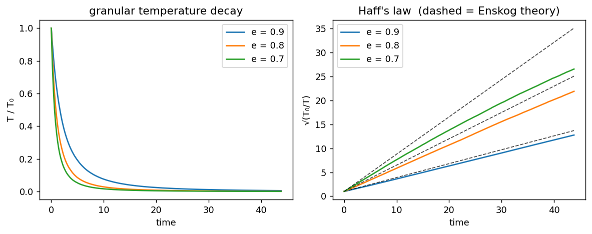
The measured cooling rate sits within ~8% of the parameter-free kinetic-theory value at e = 0.9 and tracks the (1 − e²) scaling across the board — the deviation growing at strong inelasticity exactly where Enskog’s near-elastic, molecular-chaos assumptions begin to fail.
Add the gas: a second energy sink
The MFIX-Exa case is gas–solid. Turn the gas on (a periodic fluid at rest, coupled through the drag correlation of Tang et al. (Tang et al. 2015)) and it drains the fluctuating energy far faster than collisions alone — the granular temperature collapses.
rho_g, mu_g, rho_p = 1.0, 0.4, 8.0
m_p = rho_p*Vp; dt = 0.02
def init(seed=1, T0=9.0):
    rng = np.random.default_rng(seed)
    n1 = int(np.ceil(N**(1/3))); gl = (np.arange(n1)+0.5)*L/n1
    P = np.array(np.meshgrid(gl, gl, gl, indexing="ij")).reshape(3, -1).T[:N].astype(np.float32)
    P += rng.uniform(-0.15, 0.15, P.shape).astype(np.float32); P = np.mod(P, L)
    v = rng.normal(0, np.sqrt(T0), (N, 3)).astype(np.float32); v -= v.mean(0)
    return P, v
def dem_box(P, v, e):
    d = dem.Simulation(N+64); d.initialize(shape_type=1, radius=rp); d.set_sphere_shape(rp)
    d.set_domain((0,0,0),(L,L,L)); d.enable_periodicity(True,True,True); d.set_gravity(0,0,0)
    d.set_material_params(e,0.0,0.0); d.set_solver_iterations(6,4); d.set_dt(dt)
    d.set_positions(np.c_[P, np.full(N,1/m_p,np.float32)]); d.set_velocities(v); return d

t_dry, T_dry = runs[0.9]
P, v = init(); d = dem_box(P, v, 0.9)
s = flow.Solver(int(L), int(L), int(L)); s.set_rho(rho_g); s.set_mu(mu_g); s.set_dt(dt)
for f in range(6): s.set_domain_bc(f, 0)           # all periodic
s.set_pressure_pcg(True, 30, 1e-6)
cpl = CfdDem(s, d, fluid_dt=dt, mu=mu_g, rho=rho_g, radius=rp, drag="tang",
             dem_substeps=20, periodic=(True, True, True), move_particles=True)
Tg, tg = [granular_T(np.asarray(d.get_velocities())[:N])], [0.0]
for i in range(600):
    cpl.step()
    if i % 10 == 0: Tg.append(granular_T(np.asarray(d.get_velocities())[:N])); tg.append((i+1)*dt)
Tg, tg = np.array(Tg), np.array(tg)

fig, ax = plt.subplots(figsize=(5.2, 3.5))
ax.plot(t_dry, T_dry/T_dry[0], lw=2, label="dry — collisions only (Haff)")
ax.plot(tg, Tg/Tg[0], lw=2, label="gas-coupled (CFD–DEM)")
ax.set(xlabel="time", ylabel="T / T₀", title="the gas drains the granular temperature", xlim=(0, t_dry[-1]))
ax.legend(); plt.tight_layout()
print(f"at t = {tg[-1]:.0f}: dry T/T₀ ≈ {np.interp(tg[-1], t_dry, T_dry/T_dry[0]):.3f}, gas-coupled ≈ {Tg[-1]/Tg[0]:.3f}")
at t = 12: dry T/T₀ ≈ 0.059, gas-coupled ≈ 0.000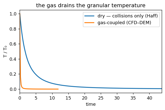
The seed of clustering
Kinetic theory assumes the gas stays uniform, but an inelastic gas does not: a slightly denser region cools faster (more collisions), loses pressure, and pulls in more grains — the clustering instability. It only grows once the box is larger than a critical wavelength, so in a modest box the effect is a slow rise of the density fluctuations above the homogeneous (Poisson) baseline rather than the dramatic clumping MFIX-Exa sees in its 256-diameter system.
Lc = 48.0; Nc = int(0.15*Lc**3/Vp); nb = 16; mu = Nc/nb**3; pois = 1/np.sqrt(mu)
def cidx(P): H = np.histogramdd(P % Lc, bins=(nb,nb,nb), range=[[0,Lc]]*3)[0]; return (H.std()/H.mean())/pois
rng = np.random.default_rng(5); n1 = int(np.ceil(Nc**(1/3))); gl = (np.arange(n1)+0.5)*Lc/n1
Pc = np.array(np.meshgrid(gl, gl, gl, indexing="ij")).reshape(3,-1).T[:Nc].astype(np.float32)
Pc += rng.uniform(-0.15, 0.15, Pc.shape).astype(np.float32); Pc = np.mod(Pc, Lc)
vc = rng.normal(0, 3, (Nc, 3)).astype(np.float32); vc -= vc.mean(0)
dc = dem.Simulation(Nc+64); dc.initialize(shape_type=1, radius=rp); dc.set_sphere_shape(rp)
dc.set_domain((0,0,0),(Lc,Lc,Lc)); dc.enable_periodicity(True,True,True); dc.set_gravity(0,0,0)
dc.set_material_params(0.4, 0.0, 0.0); dc.set_solver_iterations(6,4); dc.set_dt(dt)
dc.set_positions(np.c_[Pc, np.ones(Nc, np.float32)]); dc.set_velocities(vc)
ci, tci, snaps = [], [], []
for i in range(3600):
    dc.step(dt)
    if i % 40 == 0: ci.append(cidx(np.asarray(dc.get_positions())[:Nc])); tci.append((i+1)*dt)
    if i in (400, 3599): snaps.append(((i+1)*dt, np.asarray(dc.get_positions())[:Nc].copy()))
ci, tci = np.array(ci), np.array(tci)

fig, ax = plt.subplots(1, 3, figsize=(12, 3.7))
ax[0].plot(tci, ci); ax[0].axhline(1, ls=":", c="0.5", label="homogeneous (Poisson)")
ax[0].set(xlabel="time", ylabel="density fluctuations / Poisson", title="clustering grows (e = 0.4)"); ax[0].legend()
for k, (t, Pp) in enumerate(snaps[:2]):
    a = ax[1+k]; m = Pp[:,2] < Lc/3
    a.scatter(Pp[m,0], Pp[m,1], s=1.2, c="#333", edgecolors="none")
    a.set(title=f"t = {t:.0f}", xlim=(0,Lc), ylim=(0,Lc), aspect="equal"); a.set_xticks([]); a.set_yticks([])
plt.tight_layout()
print(f"density-fluctuation index: {ci[0]:.2f} → {ci.max():.2f}  (>1 means clustered beyond a random gas)")
density-fluctuation index: 0.38 → 1.48 (>1 means clustered beyond a random gas)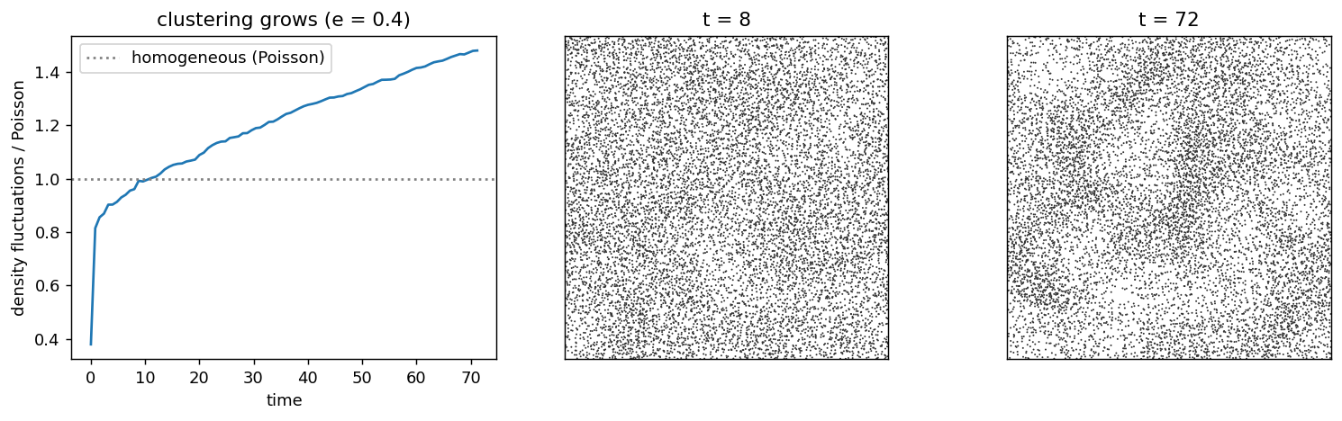
The full MFIX-Exa case — one for one
Everything above runs in a modest box to stay interactive. Now the exact benchmark: a 256 × 256 × 8 (particle-diameter) periodic domain, 50 000 grains at φ ≈ 0.05, restitution e = 0.8 (t* = t·√T₀/d_p). The benchmark is a gas–solid system, and the gas matters for more than the energy budget: interstitial drag triggers an earlier onset of the velocity-vortex and clustering instabilities than in a dry granular gas (Yin et al. 2013; Fullmer et al. 2017). The case itself is unpublished, but the MFIX-Exa input decks and source are public and fix every setting (itemised in the callout below): ρ* = 1000, ReT0 = 20, the drag correlation of Tang et al. (Tang et al. 2015) (what MFIX-Exa’s BVK2 drag option executes), smooth spheres (μ = 0), a volume-averaged incompressible gas, and a CFD grid of Δ* = 2 particle diameters. We run the case one-for-one at those settings to the benchmark’s full t* = 10 000 (make_hcs_gas_mfix.py → hcs_gas_mfix.npz), plus the dry granular system over the same range (make_hcs_mfix.py → hcs_mfix.npz) to isolate the collisional Goldhirsch–Zanetti mechanism that the gas accelerates.
data = np.load("hcs_mfix.npz")                     # dry granular run, t* = 10^4
gas = np.load("hcs_gas_mfix.npz")                  # one-for-one gas-solid run (Tang drag, Δ*=2, volume-averaged)
mfix = np.load("mfix_ref/fig33_digitized.npz")     # (t*, T/T0) traced pixel-by-pixel from Fig. 33
ts, Trat, cidx = data["ts"], data["Trat"], data["cidx"]
esm = float(data["enskog_slope"]); T0m = float(data["T0"]); Lm = float(data["Lx"])
# Two kinetic-theory (KT) curves. The benchmark's `KT` line is the GTSH result *including gas drag*:
#   dT/dt = -ζ₀(T)·T - 2·(γ(T)/m)·T,   ζ₀(T) = 2·(Enskog slope)·√(T/T₀)     (collisions + drag)
# γ(T)/m is the linear drag rate of the benchmark's own (Tang) correlation evaluated at the
# instantaneous thermal Reynolds number Re(T) = ε·√T/(μ/ρ) — parameter-free. The collisions-only
# limit (γ → 0) is Haff's law √(T₀/T) = 1 + (Enskog slope)·t.
haff = T0m/(1 + esm*ts)**2
phiM = float(data["phi"]); epsM = 1.0 - phiM; e2M = epsM*epsM; inv_e4M = 1.0/(e2M*e2M)
mu_g = 0.05; rho_g = 1.0; m_p = 1000.0*np.pi/6.0   # d_p = 1, rho_p = 1000, Re_T0 = 20
F0M = 10*phiM/e2M + e2M*(1 + 1.5*np.sqrt(phiM))    # Tang static part
def gamma_tang(T):
    Re = epsM*rho_g*np.sqrt(max(T, 1e-30))/mu_g
    F = F0M + Re*(0.11*phiM*(1+phiM) - 4.56e-3*inv_e4M + Re**-0.343*(0.169*epsM + 6.44e-2*inv_e4M))
    return 3.0*np.pi*mu_g*epsM*F/m_p
tt = np.linspace(0, ts[-1], 400000); dti = tt[1]-tt[0]; T = T0m; gt = np.empty(len(tt)); gt[0] = T0m
for k in range(1, len(tt)):
    T = max(T - (2*esm*np.sqrt(max(T, 1e-30)/T0m) + 2*gamma_tang(T))*T*dti, 1e-30); gt[k] = T
gtsh = np.interp(ts, tt, gt)
print(f"gas-solid one-for-one: N={int(gas['N'])}, φ={float(gas['phi']):.3f}, e={float(gas['e'])}, "
      f"to t*={gas['ts'][-1]:.0f}; clustering index {gas['cidx'][0]:.2f} → {gas['cidx'][-1]:.2f}. "
      f"KT at t*=1000: GTSH {np.interp(1000,ts,gtsh):.1e} vs Haff {np.interp(1000,ts,haff):.1e}")
gas-solid one-for-one: N=50000, φ=0.050, e=0.8, to t*=10000; clustering index 1.01 → 4.37. KT at t*=1000: GTSH 6.8e-05 vs Haff 4.5e-04Kinetic-energy decay — our Figure 33
The benchmark’s black KT line is the GTSH kinetic theory with the gas drag — it falls much faster than the collisions-only Haff law, reaching 10⁻⁵ near t* ≈ 10³ rather than ≈ 7×10³. Built with the same (Tang) drag law at the instantaneous thermal Reynolds number, our GTSH curve lands on the digitised MFIX KT line, and the one-for-one simulation tracks the digitised MFIX sim line through the entire run — the cooling decay, the clustering plateau, and the slow late-time decline, staying within a few tens of percent over five decades of T/T₀ and ending at 4.1×10⁻⁵ against their 6.2×10⁻⁵ at t* = 10⁴. The dry granular system cools visibly slower — the gas is a leading-order energy sink here, not a perturbation. Both simulations lift far above the homogeneous theory as the instability traps energy in coherent motion that homogeneous cooling cannot reach.
fig, ax = plt.subplots(1, 2, figsize=(11.5, 4.8))
ax[0].imshow(plt.imread("mfix_ref/hcs_ke_1908.png")); ax[0].axis("off")
ax[0].set_title("MFIX-Exa — Figure 33", fontsize=10)
m = ts >= 10; gm = gas["ts"] >= 10
ax[1].loglog(ts[m], haff[m], color="0.55", lw=1.2, label="KT — Haff (collisions only)")
ax[1].loglog(ts[m], gtsh[m], color="k", lw=1.8, label="KT — GTSH (= MFIX KT)")
ax[1].loglog(mfix["t_sim"], mfix["T_sim"], color="#d1210b", lw=2.0, alpha=0.85, label="MFIX sim (digitised)")
ax[1].loglog(gas["ts"][gm], gas["Trat"][gm], color="#2ca02c", lw=1.8, label="peclet — gas–solid (one-for-one)")
ax[1].loglog(ts[m], Trat[m], color="#1f6fb5", lw=1.5, ls="--", label="peclet — dry granular")
ax[1].set(xlabel=r"$t^* = t\,\sqrt{T_0}/d_p$", ylabel=r"$T/T_0$  or  $KE/KE_0$",
          xlim=(10, 1e4), ylim=(1e-5, 1), title="peclet vs. digitised MFIX lines")
ax[1].legend(loc="lower left", fontsize=7.5); ax[1].grid(True, which="both", alpha=0.15)
plt.tight_layout()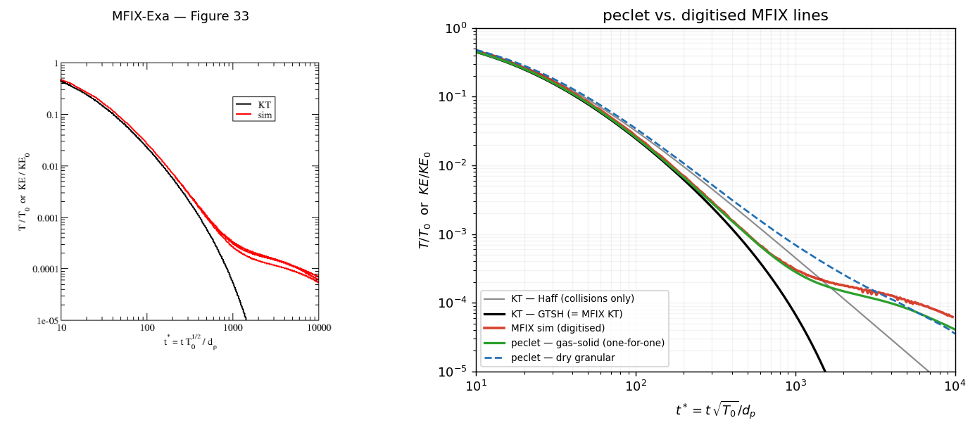
The clusters — our Figure 34
The benchmark’s Fig. 34 places the classic 2-D hard-disk computation of Goldhirsch and Zanetti (1993) (left panel) beside MFIX-Exa’s own gas–solid run (right panel, labelled t* = 1000). The energy curve above says the instability grows on schedule; the density pattern lags it: a velocity-vortex field organises first (that is what lifts the KE off the theory), and only later do the vortices sweep grains into density filaments (Fullmer and Hrenya 2017). In our one-for-one run the density texture is still faint at t* = 1000 (cluster index ≈ 1.2), sharpens into a many-filament network through t* = 2000–3000 (index 2.0 → 2.8), and keeps developing to a peak near t* ≈ 8700 (index ≈ 4.5) — the same branching-filament morphology as the benchmark panel.
fig = plt.figure(figsize=(12, 11.5))
gs = fig.add_gridspec(3, 3, height_ratios=[1.05, 1.0, 1.0], hspace=0.16, wspace=0.05)
axtop = fig.add_subplot(gs[0, :]); axtop.imshow(plt.imread("mfix_ref/hcs_xy_1908.png")); axtop.axis("off")
axtop.set_title("MFIX-Exa — Figure 34   (Goldhirsch–Zanetti 2-D reference | MFIX-Exa gas–solid result)",
                fontsize=10)
for k, tst in enumerate((2000, 5000, 10000)):
    a = fig.add_subplot(gs[1, k]); xy = gas[f"xy_{tst}"]
    a.scatter(xy[:, 0], xy[:, 1], s=0.4, c="#111", edgecolors="none")
    a.set(xlim=(0, Lm), ylim=(0, Lm), aspect="equal",
          title=f"peclet gas–solid — t* = {tst}")
    a.set_xticks([]); a.set_yticks([])
for k, tst in enumerate((2000, 5000, 10000)):
    a = fig.add_subplot(gs[2, k]); xy = data[f"xy_{tst}"]
    a.scatter(xy[:, 0], xy[:, 1], s=0.4, c="#111", edgecolors="none")
    a.set(xlim=(0, Lm), ylim=(0, Lm), aspect="equal", title=f"peclet dry — t* = {tst}")
    a.set_xticks([]); a.set_yticks([])
plt.tight_layout()
/tmp/ipykernel_402877/3143045624.py:17: UserWarning: This figure includes Axes that are not compatible with tight_layout, so results might be incorrect.
plt.tight_layout()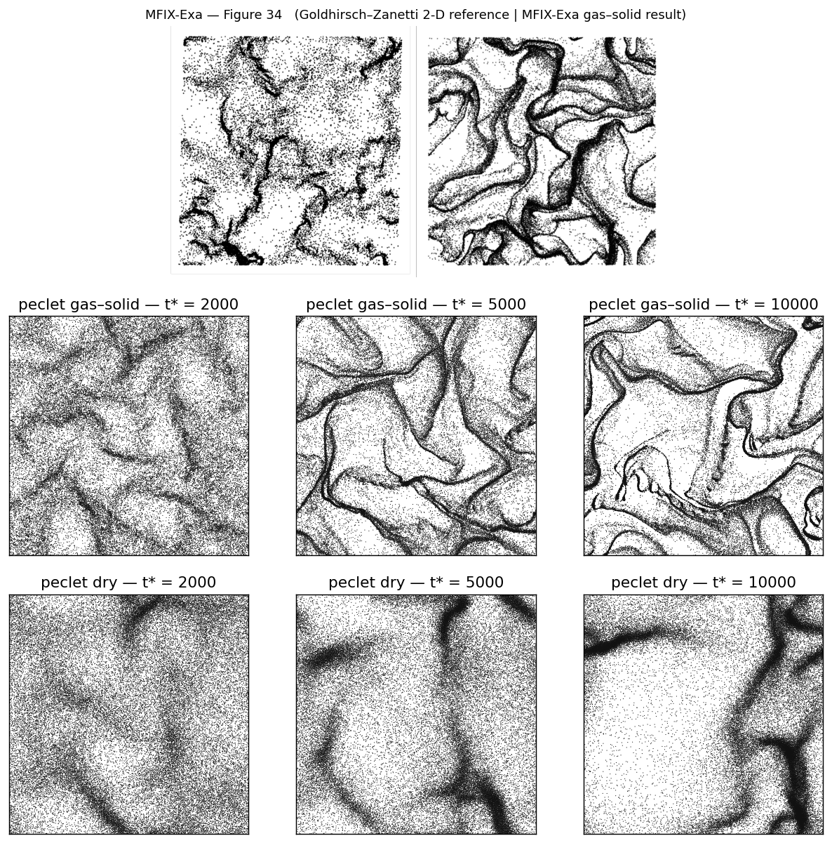
NoteThe benchmark’s settings — pinned from the MFIX-Exa sources
The 256 × 256 × 8 case itself is unpublished — the paper the benchmark cites (Fullmer et al. 2017) studies cubic boxes at φ = 0.1–0.3, and the code’s benchmarking paper (arXiv:1909.02067) covers fluidized beds — but the MFIX-Exa input decks and source code are public, and every modelling choice can be read off them. What the gas–solid run on this page matches, item by item:
- Drag. MFIX-Exa’s
BVK2drag option executes the DNS correlation of Tang et al. (Tang et al. 2015) (mfix_des_drag_K.H), with the superficial particle Reynolds number and β/n = 3πμ d ε F — the same convention implemented here (drag="tang"). - Collisions. Linear spring–dashpot with the dashpot set from ln e, so binary collisions reproduce e = 0.8 exactly by construction — as does our impulse solve. At the deck’s stiffness the contact lasts ~4 % of the mean free time (overlap ~1.6 % of dp): the soft contact is an excellent hard-sphere approximation, so the two collision models are equivalent in the binary-dominated regime that sets the cooling curve. They differ only for enduring multi-contacts inside dense filaments.
- Tangential interactions. The decks set μ = 0 and MFIX-Exa’s tangential force is Coulomb-clamped to μ|Fn| = 0 — both simulations are smooth spheres, consistent with the smooth-sphere GTSH theory both are compared against.
- Fluid. A volume-averaged incompressible gas: MFIX-Exa advects with the superficial velocity ε·u and projects ∇·(εu) = 0, with ε in all fluxes. Our run enforces the same constraint (the ∂ε/∂t term of the averaged continuity is optional in both codes and off in both runs — in MFIX-Exa by default, “under development”; here via
set_porous_deps_dt(False)). The momentum is advanced in its ε-conservative form — ερ(∂u/∂t + u·∇u) with the projection pair derived from the same inertia (the flux ε cancels the inertia ε in the Poisson coefficients). This is not a detail: with a plain-u momentum the projection drags gas along with the moving porosity at zero inertia cost and pumps particle kinetic energy without a physical source; energy consistency of the split scheme requires the ε-weighted pair. CFD grid Δ* = 2 particle diameters, per their decks and grid heuristic. - What remains — a stage offset. The fully-filamented state in the benchmark’s Fig. 34 panel, labelled t* = 1000, occurs in our run at t* ≈ 5000–10⁴, with the same branching morphology. The benchmark’s own Fig. 33 shows the KE only just plateauing at t* = 1000, which sits more comfortably with a still-developing density field than with a fully-developed network. Whether that panel corresponds to a later output or a different replicate cannot be settled from the public material; what the matched energy history (five decades, end to end), onset ordering, and morphology establish is that the instability physics is reproduced.
Results — peclet vs. theory vs. MFIX-Exa
| Prediction / benchmark | peclet | |
|---|---|---|
| Haff’s law form | √(T₀/T) linear in t (Haff 1983) |
linear (clean, all e) |
| Cooling rate | Enskog 1/t₀ ∝ (1−e²)·n·σ²·g₀·√T₀ |
within ~8% at e=0.9; tracks (1−e²) |
| Gas–solid HCS | gas drag accelerates cooling | temperature collapses well below Haff |
| Clustering | grows past a critical size (Fullmer and Hrenya 2017); gas accelerates the onset (Yin et al. 2013) | small box: fluctuations rise above Poisson; full 256-diameter box at the benchmark’s settings: KE decay on the digitised MFIX Fig. 33 sim line, branching-filament morphology of Fig. 34, gas-accelerated onset vs the dry system |
The dry granular gas reproduces Haff’s law and the Enskog cooling rate quantitatively; the gas coupling adds the second dissipation channel that makes the MFIX-Exa case gas–solid; and in the full 256-diameter box the one-for-one run lands on the benchmark’s own Fig. 33 simulation line, peels off the parameter-free GTSH theory exactly as documented, and runs away into the branching filaments of Fig. 34.
Adapt this yourself
- Raise Re_T0. Increasing the thermal Reynolds number weakens the viscous sink relative to collisions; the gas-solid HCS approaches the dry granular limit and the clustering onset moves later — sweep it and watch the KE curve migrate between the two limits shown above.
- Structure factor. Replace the coarse-grained variance with
S(k)to measure the clustering wavelength and compare to the linear-stability prediction. - Sweep the density.
g₀(φ)steepens with solids fraction — the cooling rate and the critical size both move; Equation 1 predicts how. - Different drag. The gas-damping rate depends on the drag law and the density ratio
ρ_p/ρ_g; trystokes,schiller_naumann,gidaspow.
Reproduce this
# The Haff's-law and clustering sections are pure peclet.dem and run on the PyPI wheels:
pip install peclet && quarto render examples/hcs-clustering/index.qmd --execute
# The gas-damping section needs the coupling module (built from source against a Kokkos prefix):
tools/bootstrap_deps.sh host-openmp
for m in flow dem coupling; do
  cmake -S $m -B $m/build -DCMAKE_PREFIX_PATH="$PWD/extern/install/host-openmp"; cmake --build $m/build -j
done
PECLET_LOCAL_BUILD="$PWD/flow/build:$PWD/dem/build:$PWD/coupling/build" \
  quarto render examples/hcs-clustering/index.qmd --execute
References
Fullmer, William D., and Christine M. Hrenya. 2017. “The Clustering Instability in Rapid Granular and Gas-Solid Flows.” Annual Review of Fluid Mechanics 49: 485–510. https://doi.org/10.1146/annurev-fluid-010816-060028.
Fullmer, William D., Guodong Liu, Xiaolong Yin, and Christine M. Hrenya. 2017. “Clustering Instabilities in Sedimenting Fluid-Solid Systems: Critical Assessment of Kinetic-Theory-Based Predictions Using Direct Numerical Simulation Data.” Journal of Fluid Mechanics 823: 433–69. https://doi.org/10.1017/jfm.2017.318.
Goldhirsch, Isaac, and Gianluigi Zanetti. 1993. “Clustering Instability in Dissipative Gases.” Physical Review Letters 70 (11): 1619–22. https://doi.org/10.1103/PhysRevLett.70.1619.
Haff, P. K. 1983. “Grain Flow as a Fluid-Mechanical Phenomenon.” Journal of Fluid Mechanics 134: 401–30. https://doi.org/10.1017/S0022112083003419.
Tang, Y., E. A. J. F. Peters, J. A. M. Kuipers, S. H. L. Kriebitzsch, and M. A. van der Hoef. 2015. “A New Drag Correlation from Fully Resolved Simulations of Flow Past Monodisperse Static Arrays of Spheres.” AIChE Journal 61 (2): 688–98. https://doi.org/10.1002/aic.14645.
Yin, Xiaolong, John R. Zenk, Peter P. Mitrano, and Christine M. Hrenya. 2013. “Impact of Collisional Versus Viscous Dissipation on Flow Instabilities in Gas–Solid Systems.” Journal of Fluid Mechanics 727: R2. https://doi.org/10.1017/jfm.2013.223.