import importlib.util, os, subprocess, sys
_local = os.environ.get("PECLET_LOCAL_BUILD")
if _local:
    sys.path.insert(0, _local)
elif importlib.util.find_spec("peclet") is None:
subprocess.run([sys.executable, "-m", "pip", "install", "-q", "peclet"], check=True)Lid-driven cavity vs Ghia et al. (1982)
The canonical wall-bounded benchmark: a moving lid, a primary vortex, corner eddies — matched to the classic tabulated data.
flow
boundary-conditions
verification
benchmark
 Runs on a free Colab CPU runtime — the first cell installs
 peclet from PyPI.
What you’ll learn
How to set domain boundary conditions (no-slip walls and a moving lid) with peclet, and how the solver reproduces the single most-cited incompressible-flow benchmark: the lid-driven cavity of Ghia, Ghia & Shin (1982). A square box with three stationary no-slip walls and a top lid sliding in \(+x\) drives a primary recirculating vortex plus secondary eddies in the bottom corners. We compare the centreline velocity profiles to their tabulated data at \(\mathrm{Re}=100\).
Setup
The cavity uses no immersed solid — just per-face domain BCs. Faces \(-x\), \(+x\), \(-y\) are no-slip walls (type 1); the \(+y\) lid is a Dirichlet velocity (type 2) moving at \(U\) in \(+x\). The pressure operator is the all-fluid cut-cell operator with Neumann walls (set_pressure_geometry). \(\mathrm{Re} = U L/\nu\) with \(L=N\) (grid units).
import numpy as np
import matplotlib.pyplot as plt
from peclet import flow

plt.rcParams.update({"figure.dpi": 130, "font.size": 10, "axes.grid": True,
                     "grid.alpha": 0.3, "axes.axisbelow": True,
                     "figure.facecolor": "white", "savefig.bbox": "tight"})
BLUE, RED = "#1f77b4", "#d62728"

# Ghia, Ghia & Shin (1982), Re=100: u on the vertical centreline, v on the horizontal centreline.
GHIA_Y = np.array([0, .0547, .0625, .0703, .1016, .1719, .2813, .4531, .5, .6172, .7344, .8516, .9531, .9609, .9688, .9766, 1])
GHIA_U = np.array([0, -.03717, -.04192, -.04775, -.06434, -.10150, -.15662, -.21090, -.20581, -.13641, .00332, .23151, .68717, .73722, .78871, .84123, 1])
GHIA_X = np.array([0, .0625, .0703, .0781, .0938, .1563, .2266, .2344, .5, .8047, .8594, .9063, .9453, .9531, .9609, .9688, 1])
GHIA_V = np.array([0, .09233, .10091, .10890, .12317, .16077, .17507, .17527, .05454, -.24533, -.22445, -.16914, -.10313, -.08864, -.07391, -.05906, 0])
Solve to steady state
def solve_cavity(N=64, Re=100.0, U=1.0, nz=4, dt=2.0, max_steps=2500):
    nu = U * N / Re
    s = flow.Solver(N, N, nz)
    s.set_rho(1.0); s.set_mu(nu); s.set_dt(dt); s.set_advection(True)
    s.set_domain_bc(0, 1); s.set_domain_bc(1, 1); s.set_domain_bc(2, 1)   # -x, +x, -y no-slip
    s.set_domain_bc(3, 2, U, 0.0, 0.0)                                    # +y lid moving in +x
    s.set_velocity_solver_params(60)
    s.set_pressure_multigrid(True, levels=6)
    s.set_pressure_pcg(True, 60, 1e-7)
    s.set_pressure_geometry(np.full((N, N, nz), 1e30))                    # all-fluid + Neumann walls
    prev = 0.0
    for it in range(max_steps):
        s.step()
        if it % 50 == 49:
            m = float(s.get_u()[:, :, nz // 2].mean())
            if it > 300 and abs(m - prev) < 1e-5 * (abs(m) + 1e-30):
                break
            prev = m
    u = s.get_u()[:, :, nz // 2] / U
    v = s.get_v()[:, :, nz // 2] / U
    return dict(N=N, Re=Re, u=u, v=v, steps=it + 1, div=float(s.max_open_divergence()))

r = solve_cavity()
yc = (np.arange(r["N"]) + 0.5) / r["N"]
uc = r["u"][r["N"] // 2, :]                     # u(y) on the vertical centreline
vc = r["v"][:, r["N"] // 2]                     # v(x) on the horizontal centreline
u_rms = float(np.sqrt(np.mean((np.interp(GHIA_Y, yc, uc) - GHIA_U) ** 2)))
v_rms = float(np.sqrt(np.mean((np.interp(GHIA_X, yc, vc) - GHIA_V) ** 2)))
print(f"Re={r['Re']:.0f}  N={r['N']}  ({r['steps']} steps)   u-rms vs Ghia = {u_rms:.4f}   "
      f"v-rms = {v_rms:.4f}   max divergence = {r['div']:.1e}")
Re=100 N=64 (550 steps) u-rms vs Ghia = 0.0128 v-rms = 0.0067 max divergence = 2.8e-16The cavity flow
N = r["N"]
x = (np.arange(N) + 0.5) / N
X, Y = np.meshgrid(x, x)
U2, V2 = r["u"].T, r["v"].T                      # -> shape [y, x] for streamplot
speed = np.sqrt(U2 ** 2 + V2 ** 2)

fig, ax = plt.subplots(figsize=(4.8, 4.4))
pc = ax.pcolormesh(X, Y, speed, cmap="viridis", shading="auto")
ax.streamplot(X, Y, U2, V2, color="white", density=1.3, linewidth=0.6, arrowsize=0.7)
ax.set(title=f"Lid-driven cavity, Re={r['Re']:.0f}", xlabel="x", ylabel="y", aspect="equal")
ax.grid(False)
fig.colorbar(pc, ax=ax, fraction=0.046, pad=0.04, label="|u|/U")
plt.show()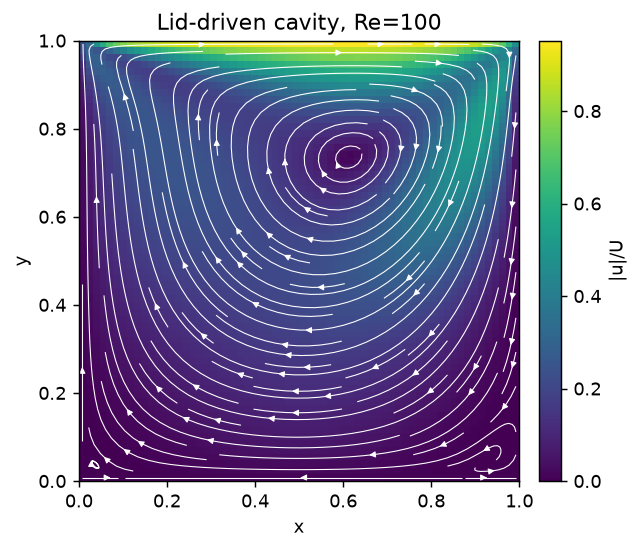
Comparison with Ghia et al.
The centreline profiles are the standard quantitative check. Our steady solution (lines) lands on the tabulated Ghia data (markers).
fig, (a0, a1) = plt.subplots(1, 2, figsize=(9, 3.9))
a0.plot(uc, yc, "-", color=BLUE, lw=1.8, label="peclet (N=64)")
a0.plot(GHIA_U, GHIA_Y, "o", color="0.15", ms=5, label="Ghia et al. 1982")
a0.set(xlabel="u / U", ylabel="y", title="vertical centreline"); a0.legend(fontsize=8)

a1.plot(x, vc, "-", color=RED, lw=1.8, label="peclet (N=64)")
a1.plot(GHIA_X, GHIA_V, "s", color="0.15", ms=5, label="Ghia et al. 1982")
a1.set(xlabel="x", ylabel="v / U", title="horizontal centreline"); a1.legend(fontsize=8)
fig.tight_layout()
plt.show()

print(f"centreline rms error vs Ghia:  u = {u_rms:.4f}   v = {v_rms:.4f}   (sub-0.02 on a 64² grid)")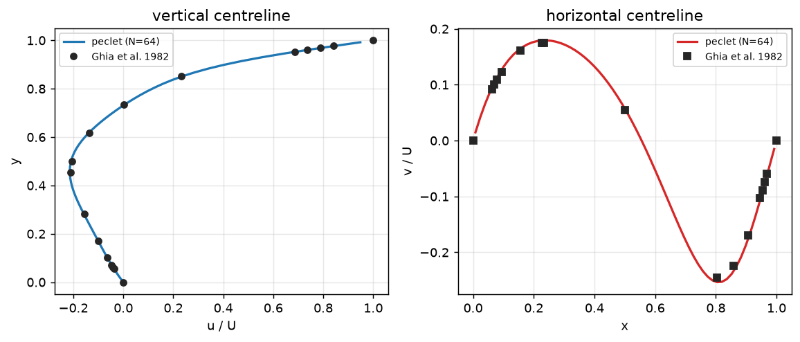
centreline rms error vs Ghia: u = 0.0128 v = 0.0067 (sub-0.02 on a 64² grid)Adapt this yourself
- Higher Reynolds number. Set
Re=400or1000(and a finer grid / more steps): the primary vortex centre migrates and the corner eddies grow — Ghia tabulate those cases too, so the comparison extends directly. - Watch it develop. Sample the field inside the loop to animate the vortex spinning up from rest.
- Deep cavity. Make the box non-square (
flow.Solver(N, 2*N, nz)) to get the stacked co-rotating vortices of a deep lid-driven cavity.
Reproduce this
pip install peclet
quarto render examples/lid-driven-cavity/index.qmd --execute
# ...or against a local source build:
PECLET_LOCAL_BUILD=/path/to/suite/flow/build_mpi OMP_NUM_THREADS=6 \
  quarto render examples/lid-driven-cavity/index.qmd --execute