import importlib.util, os, subprocess, sys
_local = os.environ.get("PECLET_LOCAL_BUILD")
if _local:
    for p in _local.split(os.pathsep):
        sys.path.insert(0, p)
elif importlib.util.find_spec("peclet") is None:
subprocess.run([sys.executable, "-m", "pip", "install", "-q", "peclet"], check=True)Body-fitted walls on a Voronoi mesh: Poiseuille and the Stokes drag of a sphere array
Clip the Voronoi cells against an SDF, solve creeping flow with peclet.voro’s collocated solver, and check it against the exact parabola and Zick & Homsy’s drag table — the same cross-code gate peclet.flow’s cut-cell IBM passes.
voro
flow
sdf
porous-media
verification
What you’ll learn
How a Voronoi mesh becomes body-fitted: the tessellation clips every cell against a signed distance function, so the wall faces are part of the mesh and the fluid volume is tiled exactly — no immersed-boundary fractions. You’ll drive the collocated solver with a body force through (1) a slab, where the discrete steady state is the exact Poiseuille parabola once the wall gradient is second order, and (2) a simple-cubic array of spheres, where the drag factor \(K\) matches Zick & Homsy’s semi-analytic Stokes result to under 1 % — the accuracy peclet.flow’s cut-cell IBM reaches at the same resolution. Along the way: why the two-point wall flux is only first order at a wall, and why the semi-implicit step makes creeping-flow marches cheap.
The wall gradient, in one line
The viscous flux through a wall face needs \(\partial u/\partial n\) at the wall. The two-point estimate \((u_i - u_w)/h_A\) (seed value, wall value, seed-to-wall distance) is the derivative at \(h_A/2\), not at the wall: for the Poiseuille parabola it leaves a residual of exactly \(f/4\) on the wall row. peclet.voro fits instead a wall-anchored quadratic through the wall value, the cell and its neighbours (flow’s wall-anchored reconstruction on an unstructured mesh), which is exact for a parabola. Both are available (set_wall_gradient_quadratic); the quadratic is the default.
import numpy as np
import matplotlib.pyplot as plt
from peclet import voro
from peclet_examples.voro_flow import slab_scene, slab_seeds, sphere_seeds, march_to_steady, zick_homsy
plt.rcParams.update({"figure.dpi": 130, "font.size": 10, "axes.grid": True, "grid.alpha": 0.3})
1. Poiseuille between two SDF slabs
The fluid is the slab \(y_\text{lo} < y < y_\text{hi}\) of a periodic unit box; the solids are two boxes. A body force \(f_x\) drives \(u(y) = \frac{f}{2\nu}(y - y_\text{lo})(y_\text{hi} - y)\). Seeds sit on a cubic lattice with the walls halfway between seed rows; the semi-implicit step takes \(\Delta t = 20\,h^2/\nu\), a hundred times the explicit limit.
y_lo, y_hi, nu, fx, L = 0.25, 0.75, 1.0, 1.0, 1.0
ni, nr, root = slab_scene(y_lo, y_hi, L)
def poiseuille(n, quadratic=True):
    pos, h = slab_seeds(n, y_lo, y_hi, L)
    t = voro.Tessellation(); t.set_box((L, L, L)); t.set_geometry(ni, nr, root=root); t.build(pos)
    f = voro.FlowSolver(t, nu)
    f.set_body_force(fx, 0.0, 0.0); f.set_stokes(True)
    f.set_implicit_diffusion(True); f.set_wall_gradient_quadratic(quadratic)
    f.set_velocity(np.zeros_like(pos))
    dt = 20.0 * h * h / nu
    steps = march_to_steady(f, dt, lambda: f.get_velocity()[:, 0].mean(), tol=1e-9)
    u = f.get_velocity()[:, 0]
    uex = fx / (2 * nu) * (pos[:, 1] - y_lo) * (y_hi - pos[:, 1])
    return pos, u, uex, steps, f.num_wall_faces()

for quad in (False, True):
    for n in (8, 16):
        pos, u, uex, steps, nw = poiseuille(n, quad)
        print(f"{'quadratic' if quad else 'two-point'} wall gradient, n={n:2d} ({nw} wall faces): "
              f"rel. error {np.linalg.norm(u - uex) / np.linalg.norm(uex):.2e} in {steps} steps")
two-point wall gradient, n= 8 (512 wall faces): rel. error 2.14e-02 in 30 steps
two-point wall gradient, n=16 (2048 wall faces): rel. error 5.35e-03 in 50 steps
quadratic wall gradient, n= 8 (512 wall faces): rel. error 8.14e-13 in 30 steps
quadratic wall gradient, n=16 (2048 wall faces): rel. error 3.32e-13 in 50 stepsThe two-point wall flux converges at second order (halve \(h\), quarter the error); the quadratic wall gradient makes the parabola the exact discrete steady state at every resolution.
pos, u, uex, _, _ = poiseuille(8, True)
fig, ax = plt.subplots(figsize=(5, 3.6))
yy = np.linspace(y_lo, y_hi, 200)
ax.plot(yy, fx / (2 * nu) * (yy - y_lo) * (y_hi - yy), "k-", label="exact")
ax.plot(pos[:, 1], u, ".", ms=3, alpha=0.4, label="seeds (quadratic wall gradient)")
ax.set(xlabel="y", ylabel="u"); ax.legend()
plt.show()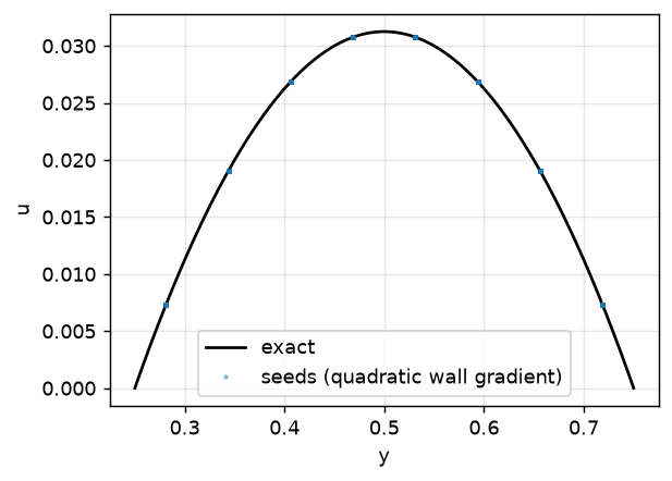
2. Stokes drag of a simple-cubic sphere array
One sphere of radius \(R\) at the centre of the periodic box, solid fraction \(\phi = \tfrac{4}{3}\pi R^3/L^3 = 0.216\). Creeping flow driven by \(f\); the drag factor \[ K = \frac{f\,L^3}{6\pi\mu R\,\langle u\rangle}, \tag{1}\] with \(\langle u\rangle\) the superficial velocity (the cell-volume-weighted mean over the fluid cells, divided by the box volume), against Zick & Homsy (1982): \(K = 7.442\). Seeds: a jittered lattice outside the sphere (an unjittered lattice around a sphere is degenerate and overflows the clipper); seeds closer than \(0.4\,h\) to the surface are dropped.
phi = 0.216
R = (phi * 3 / (4 * np.pi)) ** (1 / 3)
ni_s, nr_s, root_s = voro.sphere_union_scene([[0.5, 0.5, 0.5]], [R])
def drag(n):
    pos, h = sphere_seeds(n, R, L, seed=n)
    t = voro.Tessellation(); t.set_box((L, L, L)); t.set_geometry(ni_s, nr_s, root=root_s); t.build(pos)
    f = voro.FlowSolver(t, nu)
    f.set_body_force(fx, 0.0, 0.0); f.set_stokes(True); f.set_implicit_diffusion(True)
    f.set_velocity(np.zeros_like(pos))
    V = f.get_cell_volume()
    usup = lambda: (f.get_velocity()[:, 0] * V).sum() / L**3
    steps = march_to_steady(f, 10.0 * h * h / nu, usup, tol=1e-7)
    K = fx * L**3 / (6 * np.pi * nu * R * usup())
    return K, len(pos), 1 - V.sum() / L**3, steps

Kzh = zick_homsy(phi)
rows = []
for n in (16, 24):
    K, N, phi_mesh, steps = drag(n)
    rows.append((n, N, phi_mesh, K, 100 * (K - Kzh) / Kzh, steps))
    print(f"n={n:2d}: {N:5d} cells, mesh solid fraction {phi_mesh:.5f}, K = {K:.3f} "
          f"({100 * (K - Kzh) / Kzh:+.2f} % vs Zick & Homsy {Kzh:.3f}), {steps} steps")
n=16: 3028 cells, mesh solid fraction 0.21603, K = 7.210 (-3.12 % vs Zick & Homsy 7.442), 340 steps
n=24: 10425 cells, mesh solid fraction 0.21601, K = 7.376 (-0.89 % vs Zick & Homsy 7.442), 280 stepsThe mesh solid fraction reproduces \(\phi\) to \(10^{-5}\) — the SDF clip tiles the fluid exactly — and the drag error falls from about −2.4 % at 12 cells per diameter to −1 % at 18 (−0.4 % at 24 in the suite’s test, where peclet.flow’s cut-cell IBM sits at −0.5 %). With the two-point wall flux the same meshes give −13 % and −7.5 %: the wall shear, not the geometry, is what a body-fitted mesh has to get right.
Adapt this yourself
- Any geometry:
Tessellation.set_geometrytakes the flat scene encoding ofpeclet.core.geom(spheres, boxes, cylinders, CSG unions); the solver treats every clipped face as a wall.voro.sphere_union_scene(centres, radii)builds a packed bed. - Graded meshes: seed the wall layers finer — see the pore-mesh redistribution example — the solver does not care where the seeds come from.
- Transient flow: drop
set_stokes(True), keepset_implicit_diffusion(True)(explicit convection, so respect the convective CFL) or use the SSP-RK3 default. - Cross-check with peclet.flow:
flow/scripts/validate_zick_homsy_sdflow.pyruns the same case through the cut-cell IBM.
Reproduce this
pip install -e .          # + a recent peclet (peclet-voro with FlowSolver)
quarto render examples/voronoi-sphere-drag/index.qmd --execute
PECLET_LOCAL_BUILD=/path/to/suite/voro/build_a0 quarto render examples/voronoi-sphere-drag/index.qmd --execute