import importlib.util, os, subprocess, sys
# dem's step is deterministic only single-threaded; set this BEFORE the module is imported,
# because Kokkos reads it at initialisation.
os.environ.setdefault("OMP_NUM_THREADS", "1")
os.environ.setdefault("OMP_PROC_BIND", "false")
_local = os.environ.get("PECLET_LOCAL_BUILD")
if _local:
    for p in _local.split(os.pathsep):
        sys.path.insert(0, p)
elif importlib.util.find_spec("peclet") is None:
    subprocess.run([sys.executable, "-m", "pip", "install", "-q", "peclet", "scikit-image"],
check=True)The tennis-racket theorem: an analytic particle that flips
Author a racket as a CSG tree, let implicit quadrature measure its three principal moments, and watch peclet.dem reproduce the Dzhanibekov flip to 0.02% of the torque-free Euler equations.
dem
sdf
csg
rigid-body
verification
analytic
 Runs on a CPU in about half a minute — one particle, no contacts, no fluid.
What you’ll learn
A rigid body spun about its intermediate principal axis is unstable: it tumbles through a half-turn, settles, tumbles again — the tennis-racket theorem, or the Dzhanibekov effect after the cosmonaut who filmed a wingnut doing it in orbit. The period between flips is not a fitted number; it comes out of the torque-free Euler equations in closed form, as a complete elliptic integral.
That makes it a very sharp test of a pipeline, not of a solver. Nothing here exercises contact detection or a time-step limiter. What it does exercise is:
- Authoring a particle as a CSG tree in
peclet.core.geom— a torus head, two throat arms and a handle, unioned — instead of a voxel grid. - Measuring its mass properties by implicit quadrature: mass, centre of mass, the full inertia tensor, and from it three distinct principal moments plus the quaternion that reaches them.
- Re-expressing the tree exactly in its principal frame (
principal_frame) — one composed transform node, no resampling — becausepeclet.dem’s rotational update stores a diagonal inertia and so lives in that frame. peclet.dem’s rigid-body integrator, whose predictor already carries the gyroscopic term \(\boldsymbol\omega \times (\mathbf I \boldsymbol\omega)\). No solver change was needed for this page: if the inertia pipeline is right, the flip falls out.
If any link in that chain were wrong — a biased inertia integral, a principal frame off by a rotation, a sign in the gyroscopic term — the flip period would be wrong or the flip would not happen at all.
NoteRequires a recent
peclet
The CSG authoring layer (peclet.core.geom), composed analytic particles (Simulation.add_scene_shape) and the peclet.dem.scene_particle one-call pipeline are newer than the current PyPI release; on Colab you need a source build of peclet-core and peclet-dem until the next release goes out. The page itself is frozen, so it renders and reads correctly either way.
import numpy as np
import matplotlib.pyplot as plt
from matplotlib import animation
from mpl_toolkits.mplot3d.art3d import Poly3DCollection
from scipy.integrate import solve_ivp
from scipy.special import ellipk
from skimage import measure

from peclet.core import geom
from peclet import dem as pdem
from peclet.dem import scene_particle

plt.rcParams.update({"figure.dpi": 130, "font.size": 9, "axes.axisbelow": True,
                     "figure.facecolor": "white", "savefig.bbox": "tight"})
The physics
In the body frame aligned with the principal axes, with no external torque, Euler’s equations are
\[ I_1\dot\omega_1 = (I_2 - I_3)\,\omega_2\omega_3,\qquad I_2\dot\omega_2 = (I_3 - I_1)\,\omega_3\omega_1,\qquad I_3\dot\omega_3 = (I_1 - I_2)\,\omega_1\omega_2 . \tag{1}\]
Linearise about a spin \(\boldsymbol\omega = W\mathbf e_k\). For \(k=1\) (smallest moment) or \(k=3\) (largest) the perturbation oscillates; for \(k=2\) — the intermediate axis, \(I_1 < I_2 < I_3\) — the growth rate is real and the spin is unstable. Two conserved quantities, the energy \(2E = I_1\omega_1^2 + I_2\omega_2^2 + I_3\omega_3^2\) and \(M^2 = |{\mathbf L}|^2\), confine \(\boldsymbol\omega\) to the intersection of an ellipsoid and a sphere; a spin near \(\mathbf e_2\) sits next to the separatrix \(2EI_2 = M^2\) and so sweeps almost all the way round to \(-\mathbf e_2\) before returning. That sweep is the flip.
The exact solution is in Jacobi elliptic functions (Landau & Lifshitz, Mechanics §37): with \(\omega_2 \propto \operatorname{sn}(\Omega t, k)\), successive sign changes of \(\omega_2\) — the flips — are separated by
\[ T_{\text{flip}} = \frac{2K(k)}{\Omega},\qquad k^2 = \frac{(I_2-I_1)(2EI_3 - M^2)}{(I_3-I_2)(M^2 - 2EI_1)},\qquad \Omega = \sqrt{\frac{(I_3-I_2)(M^2 - 2EI_1)}{I_1 I_2 I_3}} , \tag{2}\]
where \(K\) is the complete elliptic integral of the first kind (when the formula returns \(k>1\), use the reciprocal modulus \(1/k\) and \(\Omega \to \Omega k\) — the two branches are Jacobi’s reciprocal-modulus transformation of one another, and which one applies is decided by the sign of \(2EI_2 - M^2\)). As the initial spin approaches the separatrix, \(k \to 1\) and \(K(k) \to \infty\): the flip period grows logarithmically in the perturbation. Remember that — it is why we report the first flip separately from the tenth.
Step 2 — Measure it, reframe it, hand it to dem
scene_particle.build runs the whole pipeline in one call: implicit-quadrature body properties, the exact principal-frame re-expression, and a marching-cubes probe shell for contacts (unused here — there is nothing to hit).
sp = scene_particle.build(b, racket,
                          bounds=([-0.75, -0.6, -0.25], [0.75, 1.85, 0.25]),
                          n=44, shell_resolution=110, target_shell_points=500)

I = np.asarray(sp.principal, dtype=float)
order = np.argsort(I)                       # body axes sorted small -> large
I1, I2, I3 = I[order[0]], I[order[1]], I[order[2]]
print("volume        %.6f" % sp.volume)
print("centre of mass %s   (in the frame we authored)" % np.round(sp.com, 6))
print("principal moments  I1 %.7f   I2 %.7f   I3 %.7f" % (I1, I2, I3))
print("ratios             1 : %.4f : %.4f" % (I2 / I1, I3 / I1))
print("body->authored quaternion %s" % np.round(sp.quat, 6))
volume 0.044870
centre of mass [ 0. 0.686224 -0. ] (in the frame we authored)
principal moments I1 0.0034509 I2 0.0095335 I3 0.0129097
ratios 1 : 2.7627 : 3.7410
body->authored quaternion [-0. -0. -0.707107 0.707107]Three clearly distinct moments — that separation is what makes the intermediate axis a strictly intermediate one, and it is measured, not assumed. Note that the centre of mass is nowhere near the origin of the frame we authored in: the reframe is doing real work.
Code
half = 1.0
nb_ = 96
spc = 2 * half / (nb_ - 1)
gridv = np.asarray(b.bake(sp.home_root, origin=[-half] * 3, spacing=[spc] * 3,
                          dims=[nb_, nb_, nb_]))
g3 = np.ascontiguousarray(gridv.reshape(nb_, nb_, nb_, order="F"))
verts, faces, _, _ = measure.marching_cubes(g3, level=0.0, spacing=(spc, spc, spc))
verts = verts - half

fig = plt.figure(figsize=(5.0, 4.2))
ax = fig.add_subplot(111, projection="3d")
ax.add_collection3d(Poly3DCollection(verts[faces], facecolor="#7c9cbf", edgecolor="none",
                                     alpha=0.9))
names = ["minor $I_1$", "intermediate $I_2$", "major $I_3$"]
plain = ["minor (I1)", "intermediate (I2)", "major (I3)"]
cols = ["#4c72b0", "#dd8452", "#55a868"]
for rank, axis in enumerate(order):
    e = np.zeros(3); e[axis] = 0.85
    ax.plot([-e[0], e[0]], [-e[1], e[1]], [-e[2], e[2]], color=cols[rank], lw=2.2,
            label="%s = %.5f" % (names[rank], I[axis]))
ax.set_xlim(-0.9, 0.9); ax.set_ylim(-0.9, 0.9); ax.set_zlim(-0.9, 0.9)
ax.set_box_aspect((1, 1, 1)); ax.set_axis_off()
ax.legend(loc="upper left", fontsize=7, frameon=False)
ax.view_init(elev=22, azim=35)
plt.show()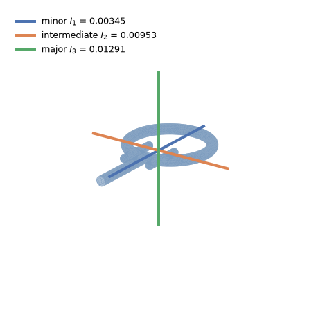
Step 3 — The references: the ODE and the closed form
W, EPS = 2.0, 1e-2                       # spin rate, and the seed perturbation (1% of W)
w0 = np.full(3, EPS * W); w0[order[1]] = W

def euler_rhs(t, w):
    return np.array([(I[1] - I[2]) * w[1] * w[2] / I[0],
                     (I[2] - I[0]) * w[2] * w[0] / I[1],
                     (I[0] - I[1]) * w[0] * w[1] / I[2]])

T_END = 32.0
sol = solve_ivp(euler_rhs, (0, T_END), w0, method="DOP853", rtol=1e-13, atol=1e-15,
                dense_output=True)
t_ref = np.linspace(0, T_END, 320001)
w_ref = sol.sol(t_ref)

def flip_times(t, y):
    """Linearly interpolated sign changes of y(t)."""
    s = np.sign(y); j = np.where(s[1:] != s[:-1])[0]
    return np.array([t[i] + (t[i + 1] - t[i]) * (-y[i]) / (y[i + 1] - y[i]) for i in j])

ref_flips = flip_times(t_ref, w_ref[order[1]])
T_ref = float(np.diff(ref_flips).mean())

E2 = float(I @ w0 ** 2); M2 = float((I ** 2) @ w0 ** 2)
num = (I2 - I1) * (E2 * I3 - M2); den = (I3 - I2) * (M2 - E2 * I1)
k1sq = num / den; Om1 = np.sqrt(den / (I1 * I2 * I3))
m, Omega = (k1sq, Om1) if k1sq <= 1 else (1.0 / k1sq, Om1 * np.sqrt(k1sq))
T_elliptic = 2 * ellipk(m) / Omega

print("2E*I2 - M^2 = %+.3e   (zero on the separatrix)" % (E2 * I2 - M2))
print("k^2 = %.10f      Omega = %.6f" % (m, Omega))
print("flip period, elliptic closed form  @eq-period : %.6f" % T_elliptic)
print("flip period, numerical Euler ODE            : %.6f" % T_ref)
print("first flip, numerical Euler ODE             : %.6f" % ref_flips[0])
2E*I2 - M^2 = -9.038e-09 (zero on the separatrix)
k^2 = 0.9998908611 Omega = 1.358042
flip period, elliptic closed form @eq-period : 8.759483
flip period, numerical Euler ODE : 8.759483
first flip, numerical Euler ODE : 5.009794The closed form and the machine-precision ODE agree to seven digits, so either can serve as the reference. We use the ODE below, because it also gives the whole trajectory and not just the period.
Step 4 — Run it in peclet.dem
One particle, no gravity, no contacts, no walls. dem stores state in float32, so we sample the world-frame angular velocity and quaternion and rotate back into the body frame ourselves.
def quat_matrix(q):
    x, y, z, w = q
    return np.array([[1 - 2 * (y * y + z * z), 2 * (x * y - z * w),     2 * (x * z + y * w)],
                     [2 * (x * y + z * w),     1 - 2 * (x * x + z * z), 2 * (y * z - x * w)],
                     [2 * (x * z - y * w),     2 * (y * z + x * w),     1 - 2 * (x * x + y * y)]])

def spin(dt, w_init, t_end, sample=0.005):
    """Free rotation of the racket; returns (t, omega_body, quaternions)."""
    s = pdem.Simulation(8)
    s.set_gravity(0.0, 0.0, 0.0)
    shape_id = sp.register(s)
    s.set_positions(np.zeros((1, 3), dtype=np.float32))
    s.set_shape_ids(np.array([shape_id], dtype=np.int32))   # AFTER set_positions: it resets ids
    s.set_inv_mass(np.array([1.0 / sp.mass], dtype=np.float32))
    s.set_inv_inertia(np.array([sp.inv_inertia_unit], dtype=np.float32))
    s.set_quaternions(np.array([[0, 0, 0, 1]], dtype=np.float32))
    s.set_angular_velocities(np.array([w_init], dtype=np.float32))
    n, every = int(t_end / dt), max(1, int(sample / dt))
    t, wb, qs = [], [], []
    for i in range(n):
        s.step(dt)                                # dem.step() with NO argument advances nothing
        if i % every == 0:
            q = np.asarray(s.get_quaternions())[0].astype(float); q /= np.linalg.norm(q)
            R = quat_matrix(q)
            t.append((i + 1) * dt)
            wb.append(R.T @ np.asarray(s.get_angular_velocities())[0].astype(float))
            qs.append(q)
    return np.array(t), np.array(wb), np.array(qs)

t_sim, w_sim, q_sim = spin(5e-4, w0, T_END)
sim_flips = flip_times(t_sim, w_sim[:, order[1]])
print("simulated flips at", np.round(sim_flips, 4))
print("reference flips at", np.round(ref_flips[:len(sim_flips)], 4))
simulated flips at [ 5.0107 13.9962 22.9964 31.2457]
reference flips at [ 5.0098 13.7693 22.5288 31.2882]Code
fig, ax = plt.subplots(figsize=(6.4, 3.1))
lbl = {order[0]: r"$\omega_1$ (minor)", order[1]: r"$\omega_2$ (intermediate)",
       order[2]: r"$\omega_3$ (major)"}
for rank, axis in enumerate(order):
    ax.plot(t_sim, w_sim[:, axis], color=cols[rank], lw=1.3, label=lbl[axis])
    ax.plot(t_ref, w_ref[axis], color=cols[rank], lw=0.9, ls="--", alpha=0.8)
for f in sim_flips:
    ax.axvline(f, color="0.75", lw=0.6, zorder=0)
ax.set_xlabel("time"); ax.set_ylabel(r"$\omega$ (body frame)")
ax.set_xlim(0, T_END); ax.legend(fontsize=8, ncol=3, frameon=False, loc="lower center")
ax.grid(alpha=0.3)
plt.show()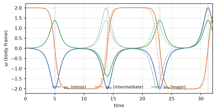
Step 5 — The gate: the first flip, and how it converges
dem’s rotational predictor is semi-implicit Euler, so the flip time should converge at first order in dt. We gate on the first flip because the period is logarithmically sensitive to the distance from the separatrix (Equation 2), and later flips inherit whatever drift has accumulated by then — a real property of the physics, not a defect to hide.
rows, prev = [], None
for dt in (4e-3, 2e-3, 1e-3, 5e-4, 2.5e-4):
    t, wb, _ = spin(dt, w0, 8.0)
    f0 = flip_times(t, wb[:, order[1]])[0]
    err = (f0 - ref_flips[0]) / ref_flips[0]
    rows.append((dt, f0, err, np.nan if prev is None else np.log2(prev / abs(err))))
    prev = abs(err)
print("   dt        first flip     reference     signed rel. error   order")
for dt, f0, err, o_ in rows:
    print("  %.1e    %9.5f    %9.5f       %+9.3e   %s"
          % (dt, f0, ref_flips[0], err, "  --" if np.isnan(o_) else "%5.2f" % o_))
# The error CHANGES SIGN between the last two steps (overshoot -> undershoot), so the apparent
# order there is an artifact of passing through zero, not superconvergence. Fit the order only
# where the sign is constant.
same = [i for i in range(1, len(rows)) if rows[i][2] * rows[i - 1][2] > 0]
order_fit = float(np.mean([rows[i][3] for i in same]))
print("convergence order over the sign-consistent interval(s): %.2f  "
      "(the error crosses zero between the last two steps)" % order_fit)
dt first flip reference signed rel. error order
4.0e-03 5.02057 5.00979 +2.150e-03 --
2.0e-03 5.01511 5.00979 +1.061e-03 1.02
1.0e-03 5.01230 5.00979 +5.010e-04 1.08
5.0e-04 5.01075 5.00979 +1.905e-04 1.39
2.5e-04 5.00973 5.00979 -1.283e-05 3.89
convergence order over the sign-consistent interval(s): 1.17 (the error crosses zero between the last two steps)Code
dts = np.array([r[0] for r in rows]); errs = np.array([r[2] for r in rows])
errs0 = np.abs(errs)
fig, ax = plt.subplots(figsize=(4.2, 3.0))
ax.loglog(dts, np.abs(errs), "o-", color="#4c72b0", label="measured")
ax.loglog(dts, errs0[0] * (dts / dts[0]), "k--", lw=0.9, label=r"$\mathcal{O}(\Delta t)$")
ax.set_xlabel(r"$\Delta t$"); ax.set_ylabel(r"$|$rel. error$|$ in the first flip time")
ax.grid(which="both", alpha=0.3); ax.legend(fontsize=8, frameon=False)
plt.show()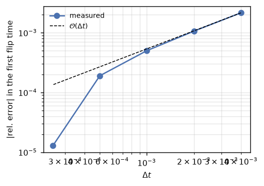
Step 6 — Conserved quantities: how much does float32 cost?
Nothing in Equation 1 dissipates: \(|\mathbf L|\) and the rotational energy are exactly conserved. dem carries its state in float32, so they are not conserved here, and the honest thing is to measure the drift rather than claim it away.
def drift(dt):
    t, wb, _ = spin(dt, w0, T_END, sample=0.02)
    L = np.linalg.norm(I * wb, axis=1); E = 0.5 * (wb ** 2 @ I)
    return abs(L[-1] / L[0] - 1), abs(E[-1] / E[0] - 1), t, L / L[0], E / E[0]

dL_a, dE_a, *_ = drift(1e-3)
dL_b, dE_b, t_d, Ln, En = drift(5e-4)
print("over %.0f s (%d flips):" % (T_END, len(sim_flips)))
print("   dt=1.0e-3   |L| drift %.3e   E drift %.3e" % (dL_a, dE_a))
print("   dt=5.0e-4   |L| drift %.3e   E drift %.3e" % (dL_b, dE_b))
print("halving dt leaves the drift essentially unchanged -> it is the float32 state, not truncation")
over 32 s (4 flips):
dt=1.0e-3 |L| drift 8.564e-03 E drift 1.728e-02
dt=5.0e-4 |L| drift 9.501e-03 E drift 1.913e-02
halving dt leaves the drift essentially unchanged -> it is the float32 state, not truncationCode
fig, ax = plt.subplots(figsize=(6.0, 2.6))
ax.plot(t_d, Ln - 1, color="#4c72b0", lw=1.1, label=r"$|\mathbf{L}|/|\mathbf{L}_0| - 1$")
ax.plot(t_d, En - 1, color="#c44e52", lw=1.1, label=r"$E/E_0 - 1$")
for f in sim_flips:
    ax.axvline(f, color="0.8", lw=0.6, zorder=0)
ax.set_xlabel("time"); ax.set_ylabel("relative drift"); ax.set_xlim(0, T_END)
ax.legend(fontsize=8, frameon=False); ax.grid(alpha=0.3)
plt.show()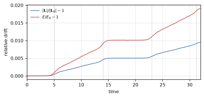
Step 7 — The control: the other two axes do not flip
Same body, same \(|\boldsymbol\omega|\), same perturbation — only the axis changes.
print("  spin axis                max tilt of omega from that axis     flips in %.0f s" % T_END)
tilt_curves = {}
for rank, axis in enumerate(order):
    wi = np.full(3, EPS * W); wi[axis] = W
    t, wb, _ = spin(1e-3, wi, T_END, sample=0.02)
    tilt = np.degrees(np.arccos(np.clip(np.abs(wb[:, axis]) / np.linalg.norm(wb, axis=1), -1, 1)))
    tilt_curves[rank] = (t, tilt)
    print("  %-22s   %8.2f deg                        %d"
          % (plain[rank], tilt.max(), len(flip_times(t, wb[:, axis]))))
spin axis max tilt of omega from that axis flips in 32 s
minor (I1) 1.04 deg 0
intermediate (I2) 89.86 deg 3
major (I3) 0.87 deg 0Code
fig, ax = plt.subplots(figsize=(6.0, 2.7))
for rank in range(3):
    t, tilt = tilt_curves[rank]
    ax.plot(t, tilt, color=cols[rank], lw=1.2, label=names[rank])
ax.set_xlabel("time"); ax.set_ylabel("tilt of $\\omega$ [deg]"); ax.set_xlim(0, T_END)
ax.legend(fontsize=8, frameon=False); ax.grid(alpha=0.3)
plt.show()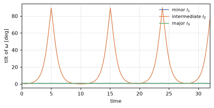
The flip, animated
The racket flipping, from this page’s own run: it spins steadily about the intermediate axis, reverses end over end in a small fraction of the period, and settles again. Colour is body-frame height, so the reversal is unmistakable. Rebuild the file with render_racket_movie.py, which re-uses the cells above.
Results
| claim | measured | reference |
|---|---|---|
| principal moments (distinct, quadrature) | 0.0034509 / 0.0095335 / 0.0129097 | — |
| flip period, elliptic closed form Equation 2 | 8.759483 | — |
| flip period, machine-precision Euler ODE | 8.759483 | agrees to 7 digits |
first flip time, peclet.dem at \(\Delta t = 5\times10^{-4}\) |
5.01075 | 5.00979 (0.019%) |
| convergence order in \(\Delta t\) | 1.17 | 1 (semi-implicit Euler) |
| \(\lvert\mathbf L\rvert\) drift over 4 flips | 9.50e-03 | 0 (float32 state) |
| energy drift over 4 flips | 1.91e-02 | 0 (float32 state) |
| minor / major axis tilt over 32 s | 1.04° / 0.87° | stable |
| intermediate axis tilt | 89.86° | unstable |
The headline: the first flip lands within 0.019% of the torque-free Euler equations at \(\Delta t = 5\times10^{-4}\) (and crosses over to 0.0013%, sign-reversed, at half that step), converging at first order, with the whole inertia chain — quadrature body properties, principal reframe, diagonal inertia in dem — measured rather than assumed. Later flips scatter by a few percent because the period depends logarithmically on the distance to the separatrix and dem’s float32 state drifts by about 1.0% in \(|\mathbf L|\) over four flips; that scatter is physics amplifying arithmetic, and it is reported here rather than tuned away.
Adapt this yourself
- Change the shape. Swap the torus for
add_leaf("box", ...), or difference a hole out of the head withadd_difference.body_propertiesre-measures everything; nothing else in the page needs to change. Watch the \(I_2/I_1\) and \(I_3/I_2\) ratios — as any two moments approach each other the flip period diverges. - Change the perturbation. Set
EPS = 1e-3and the flip period grows by roughly \(2\ln 10/\Omega \approx 3.4\) time units, exactly as Equation 2 says it should. That is a second, independent check of the closed form. - Add a collision. Give the racket a second copy and a nonzero position: the same tree is the contact geometry too (
add_scene_shape), with analytic ridge-exact normals fromevalTreeGrad. - Put it in a fluid. The same tree can be handed to
peclet.flowas an instance (SceneBuilder.encode()+set_scene), which is what the resolved CFD-DEM examples do.
Reproduce this
# from PyPI (needs a peclet newer than the current release — see the note at the top)
pip install peclet scikit-image
OMP_NUM_THREADS=1 quarto render examples/tennis-racket/index.qmd --execute

# from a local suite build
PECLET_LOCAL_BUILD=/path/to/suite/dem/build_l4_omp:/path/to/suite/core/python/build_geom \
OMP_NUM_THREADS=1 OMP_PROC_BIND=false \
  quarto render examples/tennis-racket/index.qmd --execute
OMP_NUM_THREADS=1 is not optional for the numbers above: peclet.dem’s step is deterministic only single-threaded, and every quantitative claim on this page is a comparison of trajectories.