import importlib.util, os, subprocess, sys
_local = os.environ.get("PECLET_LOCAL_BUILD")
if _local:
    for p in _local.split(os.pathsep):
        sys.path.insert(0, p)
elif importlib.util.find_spec("peclet") is None:
subprocess.run([sys.executable, "-m", "pip", "install", "-q", "peclet"], check=True)Drafting, kissing, tumbling: two spheres settling in line
Two identical spheres released one above the other in a closed box: the trailing one drafts in the leader’s wake, catches it, touches, and the pair tumbles apart side by side. The classic resolved-coupling benchmark of Fortes, Joseph & Lundgren and Glowinski et al., here as two moving analytic instances in a tank, with contact handled by the DEM.
flow
dem
coupling
moving-geometry
csg
GPU
 GPU example — the frozen page reads correctly without a solver.
What you’ll learn
Release two identical heavy spheres in line, the second a diameter behind the first. The wake of the leader lowers the drag on the follower, which accelerates and closes the gap (drafting); the two touch (kissing); the in-line configuration is unstable and the pair rotates until the spheres fall side by side (tumbling). Fortes, Joseph & Lundgren (1987) filmed it; Glowinski et al. (2001) made its three-dimensional version the standard test of resolved fluid–particle codes: two spheres of diameter \(d = 1/6\) cm, \(\rho_s/\rho_f = 1.14\), \(\mu = 0.01\) Pa·s in a \(1 \times 1 \times 4\) cm box, released at heights 3.5 and 3.16 cm.
Everything in that sentence maps onto things the previous pages validated one at a time: two moving instances with per-body reaction forces and torques (the attribution fix exists because of the second body), a closed tank built as a CSG difference (with its slab no wider than the box — the periodic-image trap), the virtual-mass stabilised coupling at a density ratio near one, and peclet.dem for the moment the spheres touch. What is new is that nothing here is prescribed: both bodies move under the forces the fluid returns, and the tumble emerges from a lateral perturbation of half a percent of a diameter.
NoteWhat is and is not claimed
The pattern — drafting, contact, tumbling into a side-by-side pair — and its internal timing are measured below. Glowinski et al. publish trajectories, not tables; without digitised curves the page does not claim a quantitative match to them, and at this resolution (\(d/h = 12\), terminal Reynolds number of a few hundred) the wake is resolved only qualitatively. The quantitative content here is the sequence, the contact time relative to the fall, and the closure of the per-body force budget — stated as such.
import time
import numpy as np
import matplotlib.pyplot as plt
from peclet import flow as sdflow
from peclet import dem as pdem
from peclet.core import geom

plt.rcParams.update({"figure.dpi": 130, "font.size": 9, "axes.axisbelow": True,
                     "figure.facecolor": "white", "savefig.bbox": "tight"})

# Glowinski et al. (2001), 3-D case, CGS
D_SI, RHO_F, RHO_S, MU_SI, G_SI = 1.0 / 6.0, 1.0, 1.14, 0.01, 981.0
BOX_SI = (1.0, 4.0, 1.0)                 # x, y (vertical), z in cm
Y1_SI, Y2_SI = 3.5, 3.16                 # release heights of the leader (lower) and follower
KI_I, KI_R = 2, 17
Kokkos::OpenMP::initialize WARNING: OMP_PROC_BIND environment variable not set
In general, for best performance with OpenMP 4.0 or better set OMP_PROC_BIND=spread and OMP_PLACES=threads
For best performance with OpenMP 3.1 set OMP_PROC_BIND=true
For unit testing set OMP_PROC_BIND=false
Kokkos::OpenMP::initialize WARNING: OMP_PROC_BIND environment variable not set
In general, for best performance with OpenMP 4.0 or better set OMP_PROC_BIND=spread and OMP_PLACES=threads
For best performance with OpenMP 3.1 set OMP_PROC_BIND=true
For unit testing set OMP_PROC_BIND=false
The setup, in dynamic similarity
The velocity scale is a nominal terminal velocity; the Reynolds number and the dimensionless gravity are then matched, as on the settling-sphere page. The sphere below (the leader) starts at 3.16 cm, the follower at 3.5 cm — one diameter of clear gap. The follower is offset laterally by \(0.005\,d\): an in-line pair is an unstable equilibrium and would otherwise tumble on round-off, in a direction set by the grid.
def run(DH, steps_max=4000, offset=0.005, adv_scheme=1):
    RATIO = RHO_S / RHO_F
    u_st = (RHO_S - RHO_F) * G_SI * D_SI ** 2 / (18 * MU_SI)      # Stokes terminal, cm/s (an upper bound)
    U_NOM = 0.3 * u_st                                              # nominal terminal (Newton-regime)
    RE = RHO_F * U_NOM * D_SI / MU_SI
    USTAR = 0.04                                                    # U_NOM in cells per time unit
    NU = USTAR * DH / RE
    GSTAR = G_SI * D_SI / U_NOM ** 2 * USTAR ** 2 / DH
    h = D_SI / DH                                                   # cm per cell
    WALL = 4.3
    NX = int(np.ceil((BOX_SI[0] / h + 2 * WALL) / 8) * 8)
    NY = int(np.ceil((BOX_SI[1] / h + 2 * WALL) / 8) * 8)
    WX = (NX - BOX_SI[0] / h) / 2; WY = (NY - BOX_SI[1] / h) / 2
    OFF = 0.3
    dt = 0.3 / USTAR / 2.0                                          # ~0.15 cell per step at U_NOM
    b = geom.SceneBuilder()
    slab = b.add_leaf("box", [NX / 2 + 1.0, NY / 2 + 1.0, NX / 2 + 1.0])   # half the box + wall: never wider
    cav = b.add_leaf("box", [(NX - 2 * WX) / 2, (NY - 2 * WY) / 2, (NX - 2 * WX) / 2])
    tank = b.add_difference(slab, cav)
    sph = b.add_leaf("sphere", [DH / 2])
    ni, nr, _, _ = b.encode()
    x0 = 0.5 * NX + OFF
    y_floor = WY + OFF
    p1 = np.array([x0, y_floor + Y2_SI / h, x0])                    # leader (lower)
    p2 = np.array([x0 + offset * DH, y_floor + Y1_SI / h, x0])      # follower, nudged in x
    ii = np.zeros((3, KI_I), dtype=np.int32); ir = np.zeros((3, KI_R))
    ii[0] = (tank, -1); ir[0, 0:3] = (0.5 * NX + OFF, 0.5 * NY + OFF, 0.5 * NX + OFF)
    ii[1] = (sph, -1); ir[1, 0:3] = p1
    ii[2] = (sph, -1); ir[2, 0:3] = p2
    ir[:, 6] = 1.0; ir[:, 7] = 1.0
    s = sdflow.Solver(NX, NY, NX)
    s.set_rho(1.0); s.set_mu(NU); s.set_dt(dt); s.set_advection(True); s.set_advection_scheme(adv_scheme)
    s.set_velocity_solver_params(60); s.set_pressure_solver_params(20)
    s.set_pressure_multigrid(True, levels=4)
    s.set_scene(np.asarray(ni, np.int32), np.asarray(nr, float), ii.ravel(), ir.ravel(), periodic=True)
    s.set_solid_from_scene(True)
    assert s.periodic_image_overlap_cells() == 0

    m = RATIO * (np.pi / 6) * DH ** 3
    Vp = (np.pi / 6) * DH ** 3
    ma = 2.0 * Vp                                                   # virtual-mass stabiliser (settling page)
    I = 0.4 * m * (DH / 2) ** 2
    d = pdem.Simulation(8)
    d.set_gravity(0.0, 0.0, 0.0)
    d.set_sphere_shape(DH / 2)
    d.set_positions(np.array([p1, p2], dtype=np.float32))
    d.set_inv_mass(np.array([1.0 / (m + ma)] * 2, dtype=np.float32))
    d.set_inv_inertia(np.array([[1.0 / I] * 3] * 2, dtype=np.float32))
    Fg = (RATIO - 1.0) * Vp * GSTAR
    a_prev = np.zeros((2, 3)); tr = []; t0 = time.time()
    for k in range(steps_max):
        P = np.asarray(d.get_positions()).astype(float)
        V = np.asarray(d.get_velocities()).astype(float)
        W = np.asarray(d.get_angular_velocities()).astype(float)
        for j in range(2):
            s.set_instance_transform(1 + j, P[j].tolist())
            s.set_instance_motion(1 + j, lin_vel=V[j].tolist(), ang_vel=W[j].tolist())
        s.rebuild_geometry(); s.step()
        FT = np.asarray(s.hydro_force_torque_reaction()).astype(float)
        F = FT[0][1:3].copy(); T = FT[1][1:3].copy()
        F[:, 1] -= Fg
        F += ma * a_prev
        d.set_external_forces(F.astype(np.float32)); d.set_external_torques(T.astype(np.float32))
        for _ in range(10):
            d.step(dt / 10)
        Vn = np.asarray(d.get_velocities()).astype(float)
        a_prev = (Vn - V) / dt
        gap = np.linalg.norm(P[1] - P[0]) - DH                         # surface-to-surface
        tr.append(((k + 1) * dt, P[0, 1], P[1, 1], P[0, 0], P[1, 0], V[0, 1], V[1, 1], gap))
        if min(P[0, 1], P[1, 1]) - y_floor < 0.75 * DH:
            break
    tr = np.array(tr)
    t_scale = h / (U_NOM / USTAR)                                       # seconds per time unit
    return dict(t=tr[:, 0] * t_scale, y=(tr[:, 1:3] - y_floor) * h, x=(tr[:, 3:5] - x0) * h,
                v=tr[:, 5:7] * (U_NOM / USTAR), gap=tr[:, 7] / DH, DH=DH, Re=RE, nstep=len(tr),
                wall=time.time() - t0, grid=(NX, NY, NX), dt_s=dt * t_scale)
r = run(12)
t, y, x, v, gap = r["t"], r["y"], r["x"], r["v"], r["gap"]
kiss = np.argmax(gap < 0.02) if (gap < 0.02).any() else None
lat = np.abs(x[:, 1] - x[:, 0]) / D_SI
side = np.argmax(lat > 0.8) if (lat > 0.8).any() else None
print("grid %dx%dx%d d/h=%d nominal Re=%.0f steps=%d dt=%.2e s wall %.0f s"
% (*r["grid"], r["DH"], r["Re"], r["nstep"], r["dt_s"], r["wall"]))
print(" follower faster than leader from t = %.3f s (drafting)" % t[np.argmax(-v[:, 1] > -v[:, 0] + 0.02 * abs(v[:, 0]).max())])
print(" contact (gap < 0.02 d) at t = %s" % ("%.3f s" % t[kiss] if kiss is not None else "never"))
print(" side by side (|dx| > 0.8 d) at t = %s" % ("%.3f s" % t[side] if side is not None else "never"))
print(" peak settling speeds: leader %.2f cm/s, follower %.2f cm/s" % (-v[:, 0].min(), -v[:, 1].min()))grid 88x304x88 d/h=12 nominal Re=106 steps=1960 dt=3.28e-04 s wall 1580 s
follower faster than leader from t = 0.153 s (drafting)
contact (gap < 0.02 d) at t = 0.333 s
side by side (|dx| > 0.8 d) at t = 0.482 s
peak settling speeds: leader 6.05 cm/s, follower 8.48 cm/sCode
fig, ax = plt.subplots(1, 3, figsize=(9.6, 3.0))
ax[0].plot(t, y[:, 0], color="#4c72b0", label="leader"); ax[0].plot(t, y[:, 1], color="#c44e52", label="follower")
a0b = ax[0].twinx(); a0b.plot(t, gap, color="#8c8c8c", lw=0.9, ls=":"); a0b.set_ylabel("gap / d", color="#8c8c8c"); a0b.set_ylim(-0.05, 1.3)
ax[0].set_xlabel("t [s]"); ax[0].set_ylabel("height [cm]"); ax[0].legend(fontsize=8, frameon=False)
ax[1].plot(t, -v[:, 0], color="#4c72b0"); ax[1].plot(t, -v[:, 1], color="#c44e52")
ax[1].set_xlabel("t [s]"); ax[1].set_ylabel("settling speed [cm/s]")
ax[2].plot(t, lat, color="#55a868"); ax[2].set_xlabel("t [s]"); ax[2].set_ylabel("|x₂ − x₁| / d")
for a in ax:
    a.grid(alpha=0.3)
    if kiss is not None: a.axvline(t[kiss], color="k", lw=0.6, ls="--")
plt.tight_layout(); plt.show()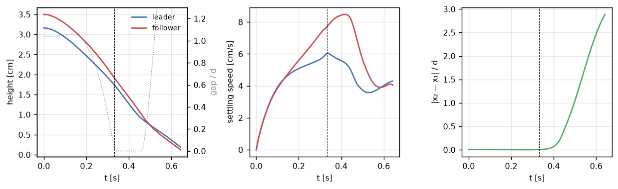
Results
| claim | measured | reference |
|---|---|---|
| drafting: follower faster than leader before contact | yes | Fortes et al. (1987) |
| contact time | 0.333 s | Glowinski et al. (2001): within the first half of the fall |
| tumbling: lateral separation reaches 0.8 d | 0.482 s | side-by-side pair, the stable end state |
| peak speed vs Schiller–Naumann terminal | 6.0 / 8.5 cm/s | drafting follower exceeds a single sphere’s terminal |
| periodic-image overlap of the tank | 0 cells (asserted) | the slab rule |
Adapt this yourself
- Refine. \(d/h = 16\) quadruples the cost and starts to resolve the leader’s wake at these Reynolds numbers; the contact time is the number to watch.
- Three spheres, or a row. More instances are more rows in
ii/irand a longer dem array — the attribution and the contact model do not care. - Friction and restitution. The contact here is frictionless and inelastic by dem’s default;
set_material_paramsandset_restitution_modelchange what happens at the kiss.
Reproduce this
PECLET_LOCAL_BUILD=/path/to/suite/flow/build_l3_cuda:/path/to/suite/dem/build_l4_cuda:/path/to/suite/core/python/build_geom \
  quarto render examples/drafting-kissing-tumbling/index.qmd --execute
References
Fortes, A. F., D. D. Joseph, and T. S. Lundgren. 1987. “Nonlinear Mechanics of Fluidization of Beds of Spherical Particles.” Journal of Fluid Mechanics 177: 467–83. https://doi.org/10.1017/S0022112087001046.
Glowinski, R., T.-W. Pan, T. I. Hesla, D. D. Joseph, and J. Périaux. 2001. “A Fictitious Domain Approach to the Direct Numerical Simulation of Incompressible Viscous Flow Past Moving Rigid Bodies: Application to Particulate Flow.” Journal of Computational Physics 169 (2): 363–426. https://doi.org/10.1006/jcph.2000.6542.