import importlib.util, os, subprocess, sys
_local = os.environ.get("PECLET_LOCAL_BUILD")
if _local:
    for p in _local.split(os.pathsep):
        sys.path.insert(0, p)
elif importlib.util.find_spec("peclet") is None:
subprocess.run([sys.executable, "-m", "pip", "install", "-q", "peclet"], check=True)A sphere that really moves: does the drag spike?
Sharp-interface immersed boundaries are known to produce spurious force oscillations when a body crosses grid cells. Here is how big they are in peclet.flow, where they come from, and the one-line change that removes them.
flow
IBM
moving-geometry
verification
drag
GPU
 GPU example — the frozen page reads correctly without a solver.
What you’ll learn
The oscillating sphere never moved. Its boundary condition oscillated while the geometry stayed put, which is the linearised limit, and in that limit the complex drag matches Stokes (1851) to 0.23%.
Let the sphere actually translate through the fixed grid and something else appears. As the surface sweeps across cell faces, cells emerge from the body and the discrete stencil changes abruptly. Both events are discontinuous in time, and both land in the force. The result is the spurious force oscillation — a well-documented pathology of immersed-boundary methods (Lee et al. 2011; Seo and Mittal 2011; Uhlmann 2005), and a serious one for resolved CFD-DEM, where that force is the coupling.
So: how big is it here, what causes it, and can it be fixed? This page answers all three, and it does so with two references that leave nowhere to hide:
- An exact internal one. At the same parameters, the linearised run — boundary condition moving, geometry static — is the same physical problem without any interface motion. Its residual is the floor. Anything above that floor is what the motion introduced.
- An external one beyond Stokes. With advection on, Blackburn (2002) tabulates peak drag coefficients for a sphere oscillating in quiescent fluid across amplitude and Reynolds number, computed spectrally.
NoteRequires a recent
peclet
The analytic-scene API, hydro_force_torque_reaction and set_fresh_cell_seed are newer than the current PyPI release. The page is frozen and renders regardless.
import time
import numpy as np
import matplotlib.pyplot as plt
from peclet import flow as sdflow

plt.rcParams.update({"figure.dpi": 130, "font.size": 9, "axes.axisbelow": True,
                     "figure.facecolor": "white", "savefig.bbox": "tight"})
RHO, MU = 1.0, 0.1
NU = MU / RHO
KN_R, KI_I, KI_R = 16, 2, 17
Kokkos::OpenMP::initialize WARNING: OMP_PROC_BIND environment variable not set
In general, for best performance with OpenMP 4.0 or better set OMP_PROC_BIND=spread and OMP_PLACES=threads
For best performance with OpenMP 3.1 set OMP_PROC_BIND=true
For unit testing set OMP_PROC_BIND=false
The two mechanisms
When a body moves through a fixed grid, two things happen that do not happen when it is still.
- Fresh cells. A cell the body has just uncovered has no fluid history. Whatever the solver restores there is a guess. Restoring the value the solid held — zero, or a stale masked value — hands a point that should be moving with the wall a state that says it is at rest, and the discrete reaction charges the body for the difference.
- Stencil switching. As the interface crosses a face, the cut-cell coefficients change by a finite amount in one step. That is a genuine discontinuity in the discrete operator.
Both are spatial in origin, and that has a sharp consequence which the measurements below exploit: refining the time step does not help. It cannot — the events are triggered by the geometry, not the clock — and a finer time step actually makes each jump look sharper.
Measuring it
We use two metrics, deliberately.
\[ \mathrm{RMS}\!\left(\left|F^{n+1} - 2F^{n} + F^{n-1}\right|\right) \Big/ |\hat F_1| \tag{1}\]
is the second-difference measure of Seo & Mittal (2011, Eq. 12), the one the literature actually uses (Martins et al. (2017) adopt it verbatim). It is a high-pass filter: it passes step-to-step jumps and crushes the driving frequency.
\[ \text{residual} = F(t) - \sum_{m=0}^{5} \left[a_m \cos m\omega t + b_m \sin m\omega t\right] \tag{2}\]
is what is left after removing the first five harmonics of the driving frequency — flat spectral gain, no explicit \(\Delta t\) dependence of its own, and directly interpretable as the part of the force that is not at the driving frequency. We report both, and they legitimately disagree about the time-step exponent, because Equation 1 carries an \((\omega\Delta t)^2\) rolloff of its own.
WarningWhat is and is not comparable to published numbers
The form of Equation 1 is the literature’s. The absolute value is not: we normalise by the fundamental force amplitude, not by Seo & Mittal’s \(C_{PD}\). And their reported exponents come from a 2-D cylinder, where the swept-volume argument scales as \(\Delta x^2/\Delta t\); ours is a 3-D sphere, where it is \(\Delta x^3/\Delta t\). No exponent claimed here is a match to theirs, and a numerical coincidence between the two would not be evidence of anything.
_CACHE = {}

def run(N, R, AR, SPP, seed, moving=True, nper=3, fitp=2, dr=1.0):
    key = (N, R, AR, SPP, seed, moving, nper, fitp, dr)
    if key not in _CACHE:
        _CACHE[key] = _run(N, R, AR, SPP, seed, moving, nper, fitp, dr)
    return _CACHE[key]

def _run(N, R, AR, SPP, seed, moving, nper, fitp, dr):
    delta = dr * R
    om = 2 * NU / delta ** 2
    A = AR * R
    U0 = A * om                       # velocity amplitude follows from amplitude and frequency
    period = 2 * np.pi / om
    dt = period / SPP
    x0 = 0.5 * N
    node_ints = np.array([1, -1, -1], dtype=np.int32)
    node_reals = np.zeros(KN_R); node_reals[0] = R
    node_reals[14] = 1.0; node_reals[15] = 1.0
    inst_ints = np.zeros((1, KI_I), dtype=np.int32); inst_ints[0] = (0, -1)
    inst_reals = np.zeros((1, KI_R))
    inst_reals[0, 0:3] = (x0, 0.5 * N, 0.5 * N)
    inst_reals[0, 6] = 1.0; inst_reals[0, 7] = 1.0

    s = sdflow.Solver(N, N, N)
    s.set_rho(RHO); s.set_mu(MU); s.set_dt(dt); s.set_advection(False)
    s.set_velocity_solver_params(100); s.set_pressure_solver_params(25)
    s.set_pressure_multigrid(True, levels=4)
    s.set_scene(node_ints, node_reals, inst_ints.ravel(), inst_reals.ravel(), periodic=True)
    s.set_fresh_cell_seed(bool(seed))
    s.set_instance_motion(0, lin_vel=[U0, 0.0, 0.0])
    s.set_solid_from_scene(True)

    t, force = [], []
    t0 = time.time()
    for it in range(SPP * nper):
        now = (it + 1) * dt                     # backward Euler: the BC belongs at t^{n+1}
        u = U0 * np.cos(om * now)
        if moving:
            s.set_instance_transform(0, [x0 + A * np.sin(om * now), 0.5 * N, 0.5 * N])
            s.set_instance_motion(0, lin_vel=[u, 0.0, 0.0])
            s.rebuild_geometry()                # the body has MOVED: full re-derivation
        else:
            s.set_instance_motion(0, lin_vel=[u, 0.0, 0.0])
            s.refresh_wall_velocity()           # geometry static: only the BC moves
        s.step()
        t.append(now)
        force.append(float(np.asarray(s.hydro_force_torque_reaction())[0][0][0]))

    t = np.array(t); force = np.array(force)
    keep = t >= (nper - fitp) * period
    tk, fk = t[keep], force[keep]
    cols = [np.ones_like(tk)]
    for m in range(1, 6):
        cols += [np.cos(m * om * tk), np.sin(m * om * tk)]
    basis = np.column_stack(cols)
    coef, *_ = np.linalg.lstsq(basis, fk, rcond=None)
    res = fk - basis @ coef
    F1 = np.hypot(coef[1], coef[2])
    d2 = np.abs(fk[2:] - 2 * fk[1:-1] + fk[:-2])
    return dict(t=tk, F=fk, fit=basis @ coef, res=res, F1=F1, A=A, om=om, period=period,
                p2p=(res.max() - res.min()) / F1, rms=res.std() / F1,
                d2=float(np.sqrt((d2 ** 2).mean())) / F1, wall=time.time() - t0)
Step 1 — The headline: with and without
Same problem, three ways, at \(R/h = 9.6\), \(\delta/R = 1\), amplitude \(A = 2.4\) cells (so the surface sweeps about ten cells per cycle).
N0, R0, AR0, SPP0 = 96, 9.6, 0.25, 200
ref  = run(N0, R0, AR0, SPP0, 0, moving=False)     # geometry static: the floor
off  = run(N0, R0, AR0, SPP0, 0)                   # moving, fresh cells inherit the solid
on   = run(N0, R0, AR0, SPP0, 1)                   # moving, fresh cells seeded
print("                          |F1|          bias vs static   RMS(F_2delta)/|F1|   residual p2p/|F1|")
for tag, r in (("static (geometry fixed)", ref), ("moving, seeding OFF", off),
               ("moving, seeding ON", on)):
    bias = "     --   " if r is ref else "  %+7.2f%%" % (100 * (r["F1"] / ref["F1"] - 1))
    print("  %-24s %.5e %s        %.3e           %.3e"
          % (tag, r["F1"], bias, r["d2"], r["p2p"]))
|F1| bias vs static RMS(F_2delta)/|F1| residual p2p/|F1|
static (geometry fixed) 2.19999e-01 -- 6.975e-04 2.287e-03
moving, seeding OFF 2.25744e-01 +2.61% 3.065e-02 1.064e-01
moving, seeding ON 2.19913e-01 -0.04% 9.553e-04 5.948e-03Code
fig, (a1, a2) = plt.subplots(2, 1, figsize=(6.6, 4.4), sharex=True,
                             gridspec_kw={"height_ratios": [1, 1.1]})
cyc = (off["t"] - off["t"][0]) / off["period"]
a1.plot(cyc, ref["F"], color="0.55", lw=1.0, label="static (geometry fixed)")
a1.plot(cyc, off["F"], color="#c44e52", lw=1.0, label="moving, seeding OFF")
a1.plot(cyc, on["F"], color="#4c72b0", lw=1.0, ls="--", label="moving, seeding ON")
a1.set_ylabel("$F_x$"); a1.legend(fontsize=7.5, frameon=False, ncol=3); a1.grid(alpha=0.3)
a2.plot(cyc, ref["res"] / ref["F1"], color="0.55", lw=0.9)
a2.plot(cyc, off["res"] / off["F1"], color="#c44e52", lw=0.9)
a2.plot(cyc, on["res"] / on["F1"], color="#4c72b0", lw=0.9)
a2.set_xlabel("cycles"); a2.set_ylabel("residual / $|\\hat F_1|$"); a2.grid(alpha=0.3)
plt.tight_layout(); plt.show()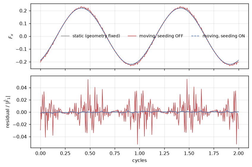
Step 2 — Refining the time step makes it worse
This is the diagnostic. A temporal discretisation error shrinks when \(\Delta t\) shrinks. A grid-crossing artefact does not — the same jumps happen, resolved more sharply.
print("  steps/cycle |  seeding OFF: RMS(F_2d)  p2p     bias  |  seeding ON: RMS(F_2d)  p2p     bias")
dt_rows = []
for spp in (100, 200, 400):
    o = run(N0, R0, AR0, spp, 0); n = run(N0, R0, AR0, spp, 1)
    r = run(N0, R0, AR0, spp, 0, moving=False)
    dt_rows.append((spp, o, n, r))
    print("     %4d     |     %.3e  %.3e  %+5.2f%%  |    %.3e  %.3e  %+5.2f%%"
          % (spp, o["d2"], o["p2p"], 100 * (o["F1"] / r["F1"] - 1),
             n["d2"], n["p2p"], 100 * (n["F1"] / r["F1"] - 1)))
print("  the static floor at every step size: RMS(F_2d) = %.3e" % ref["d2"])
steps/cycle | seeding OFF: RMS(F_2d) p2p bias | seeding ON: RMS(F_2d) p2p bias
100 | 2.804e-02 5.718e-02 +2.48% | 3.067e-03 4.853e-03 -0.16%
200 | 3.065e-02 1.064e-01 +2.61% | 9.553e-04 5.948e-03 -0.04%
400 | 4.128e-02 1.338e-01 +2.69% | 6.255e-04 5.890e-03 +0.03%
the static floor at every step size: RMS(F_2d) = 6.975e-04Step 3 — Refining the grid does help, and the bias does not
print("   N   R/h   |  seeding OFF: RMS(F_2d)   bias   |  seeding ON: RMS(F_2d)   bias  | floor")
h_rows = []
for N, R in ((64, 6.4), (96, 9.6), (128, 12.8)):
    o = run(N, R, AR0, SPP0, 0); n = run(N, R, AR0, SPP0, 1)
    r = run(N, R, AR0, SPP0, 0, moving=False)
    h_rows.append((N, R, o, n, r))
    print("  %3d  %5.1f  |     %.3e  %+6.2f%%   |    %.3e  %+6.2f%%  | %.3e"
          % (N, R, o["d2"], 100 * (o["F1"] / r["F1"] - 1),
             n["d2"], 100 * (n["F1"] / r["F1"] - 1), r["d2"]))
N R/h | seeding OFF: RMS(F_2d) bias | seeding ON: RMS(F_2d) bias | floor
64 6.4 | 6.450e-02 +2.91% | 1.557e-03 +0.38% | 6.975e-04
96 9.6 | 3.065e-02 +2.61% | 9.553e-04 -0.04% | 6.975e-04
128 12.8 | 2.126e-02 +2.71% | 8.162e-04 +0.16% | 6.975e-04The bias column without seeding is the important one: +2.9 / +2.6 / +2.7% as the grid is refined by a factor of two. It is a resolution-independent drag error — the same signature the reconstructed-traction force carries, and not something refinement will fix. With seeding it is at most a few tenths of a percent and scatters around zero.
Code
fig, (a1, a2) = plt.subplots(1, 2, figsize=(7.2, 2.9))
sp = np.array([r[0] for r in dt_rows])
a1.loglog(1.0 / sp, [r[1]["d2"] for r in dt_rows], "o-", color="#c44e52", label="seeding OFF")
a1.loglog(1.0 / sp, [r[2]["d2"] for r in dt_rows], "s-", color="#4c72b0", label="seeding ON")
a1.axhline(ref["d2"], color="0.5", ls="--", lw=0.9, label="static floor")
a1.set_xlabel(r"$\Delta t$ / cycle"); a1.set_ylabel(r"RMS$(F_{2\delta})/|\hat F_1|$")
a1.legend(fontsize=7.5, frameon=False); a1.grid(which="both", alpha=0.3)
a1.set_title("time-step leg", fontsize=9)
rr = np.array([r[1] for r in h_rows])
a2.loglog(1.0 / rr, [r[2]["d2"] for r in h_rows], "o-", color="#c44e52", label="seeding OFF")
a2.loglog(1.0 / rr, [r[3]["d2"] for r in h_rows], "s-", color="#4c72b0", label="seeding ON")
a2.loglog(1.0 / rr, [r[4]["d2"] for r in h_rows], "--", color="0.5", lw=0.9, label="static floor")
a2.set_xlabel(r"$h/R$"); a2.set_ylabel(r"RMS$(F_{2\delta})/|\hat F_1|$")
a2.legend(fontsize=7.5, frameon=False); a2.grid(which="both", alpha=0.3)
a2.set_title("grid leg", fontsize=9)
plt.tight_layout(); plt.show()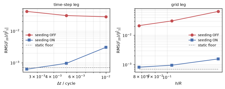
Step 4 — The fix
set_fresh_cell_seed(True) gives a just-uncovered point the local wall velocity — the rigid-body velocity of the instance that released it, evaluated at the nearest wall point, which the solver already computes for the no-slip condition. It is bounded, needs no new field, and reduces exactly to the old behaviour when nothing moves.
It does not touch the second mechanism, the stencil switch. That it works this well says the fresh cells were the dominant term here — which is what the sharp-interface literature reports too.
This is now the default in peclet.flow. The evidence was not only the force on a single body: in the resolved CFD-DEM loop, the settling-sphere gate’s total-momentum leak falls from \(1.07\times10^{-2}\) to \(1.13\times10^{-4}\) of \(F_g\) per unit time — a factor of 95.
Step 5 — Beyond Stokes: against Blackburn (2002)
Everything above is linear (advection off), where the linearised run is an exact reference. Turn advection on and neither reference applies — so we go to the literature. Blackburn (2002) computed a sphere oscillating in quiescent fluid spectrally and tabulated the peak drag coefficient, \(C_d = 8F_d/(\rho U_{\max}^2 \pi D^2)\), against \(A/D\) and \(\mathrm{Re} = U_{\max}D/\nu\). The peak is the maximum of the instantaneous curve over a cycle, not a Fourier amplitude, so we take it the same way.
The Stokes-layer thickness sets the resolution requirement: \(\delta/D = \sqrt{2(A/D)/\mathrm{Re}}\).
BLACKBURN = {(1.0, 20): 4.29, (0.5, 20): 5.70, (1.0, 50): 2.75, (0.2, 20): 9.36}

def run_fre(N, R, AD, Re, SPP=200, nper=3, seed=True):
    D = 2 * R; A = AD * D
    Umax = Re * NU / D
    om = Umax / A; period = 2 * np.pi / om; dt = period / SPP
    delta = D * np.sqrt(2 * AD / Re)
    x0 = 0.5 * N
    node_ints = np.array([1, -1, -1], dtype=np.int32)
    node_reals = np.zeros(KN_R); node_reals[0] = R
    node_reals[14] = 1.0; node_reals[15] = 1.0
    inst_ints = np.zeros((1, KI_I), dtype=np.int32); inst_ints[0] = (0, -1)
    inst_reals = np.zeros((1, KI_R)); inst_reals[0, 0:3] = (x0, 0.5 * N, 0.5 * N)
    inst_reals[0, 6] = 1.0; inst_reals[0, 7] = 1.0
    s = sdflow.Solver(N, N, N)
    s.set_rho(RHO); s.set_mu(MU); s.set_dt(dt)
    s.set_advection(True)                       # finite Re: the reaction budget carries it
    s.set_velocity_solver_params(100); s.set_pressure_solver_params(25)
    s.set_pressure_multigrid(True, levels=4)
    s.set_scene(node_ints, node_reals, inst_ints.ravel(), inst_reals.ravel(), periodic=True)
    s.set_fresh_cell_seed(seed)
    s.set_instance_motion(0, lin_vel=[Umax, 0.0, 0.0])
    s.set_solid_from_scene(True)
    t, force, umean = [], [], []
    t0 = time.time()
    for it in range(SPP * nper):
        now = (it + 1) * dt
        s.set_instance_transform(0, [x0 + A * np.sin(om * now), 0.5 * N, 0.5 * N])
        s.set_instance_motion(0, lin_vel=[Umax * np.cos(om * now), 0.0, 0.0])
        s.rebuild_geometry(); s.step()
        t.append(now)
        force.append(float(np.asarray(s.hydro_force_torque_reaction())[0][0][0]))
        umean.append(float(np.asarray(s.get_u()).mean()))
    t = np.array(t); Cd = 8 * np.array(force) / (RHO * Umax ** 2 * np.pi * D ** 2)
    last = t >= (nper - 1) * period
    return dict(peak=float(np.abs(Cd[last]).max()), Cd=Cd, t=t, last=last, D=D,
                delta_h=delta, umean=np.abs(umean).max() / Umax, wall=time.time() - t0,
period=period)print(" L/D R/h delta/h | peak |Cd| Blackburn difference | |<u>|max/Umax time")
fre_rows = []
for N, R, AD, Re, tag in ((96, 6.4, 1.0, 20, "box arm"), (128, 6.4, 1.0, 20, ""),
(160, 8.0, 1.0, 20, ""), (200, 10.0, 1.0, 20, ""),
(200, 10.0, 0.5, 20, "different amplitude")):
r = run_fre(N, R, AD, Re)
ref_cd = BLACKBURN[(AD, Re)]
fre_rows.append((N, R, AD, Re, r, ref_cd))
print(" %4.1f %5.1f %6.2f | %.4f %.2f %+6.2f%% | %.4f %4.0f s %s"
% (N / (2 * R), R, r["delta_h"], r["peak"], ref_cd,
100 * (r["peak"] / ref_cd - 1), r["umean"], r["wall"], tag)) L/D R/h delta/h | peak |Cd| Blackburn difference | |<u>|max/Umax time
7.5 6.4 4.05 | 4.2572 4.29 -0.76% | 0.0042 72 s box arm
10.0 6.4 4.05 | 4.2617 4.29 -0.66% | 0.0018 144 s
10.0 8.0 5.06 | 4.1987 4.29 -2.13% | 0.0018 260 s
10.0 10.0 6.32 | 4.1971 4.29 -2.17% | 0.0018 564 s
10.0 10.0 4.47 | 5.6689 5.70 -0.54% | 0.0012 564 s different amplitudeThe first two rows differ only in box size, \(L/D = 7.5\) against \(10\), and the peak moves by 0.1% — the periodic box is not the limitation. The domain-mean velocity stays below 0.2% of \(U_{\max}\) on the main ladder (0.5% on the smaller-box arm), which matters because a periodic box has no outflow and its mean momentum is unpinned; here it simply never grows enough to matter.
Across the whole ladder — \(\delta/h \approx 4\) to \(6.3\), where \(\delta/D = \sqrt{2(A/D)/\mathrm{Re}}\) is the Stokes layer — the peak drag now sits within about two percent of Blackburn’s spectral value, with a small negative offset that does not refine away.
NoteAn earlier version of this page read a much larger error here — and mis-read its cause
It measured +10.3% at \(\delta/h \approx 4\) decaying to within half a percent by \(\delta/h = 6.3\), and took that for the Stokes layer resolving. Most of it was something else. The momentum-advection kernels were reading the solver’s masked zeros inside the moving sphere, and zero is the wall velocity only for a wall that does not move; feeding them the rigid-body velocity instead (peclet-flow fb1a1a7) removes that error — and with it most of the apparent \(\delta/h\) trend, because what looked like convergence was largely that error decaying. The half-amplitude row is the check that what remains is not case-specific: a different \(A/D\), a different reference value, 38 rather than 77 cell crossings per cycle, and it lands in the same band. A couple of percent, flat in resolution, is an honest present limit — and no longer explicable as an unresolved boundary layer.
Code
fig, (a1, a2) = plt.subplots(1, 2, figsize=(7.2, 2.9))
N, R, AD, Re, r, ref_cd = fre_rows[3]
tt = (r["t"][r["last"]] - r["t"][r["last"]][0]) / r["period"]
a1.plot(tt, r["Cd"][r["last"]], color="#4c72b0", lw=1.2)
a1.axhline(ref_cd, color="#c44e52", ls="--", lw=1.0, label="Blackburn peak %.2f" % ref_cd)
a1.axhline(-ref_cd, color="#c44e52", ls="--", lw=1.0)
a1.set_xlabel("cycles"); a1.set_ylabel("$C_d$")
a1.set_title("$A/D=1$, Re$=20$, $\\delta/h=%.1f$" % r["delta_h"], fontsize=9)
a1.legend(fontsize=7.5, frameon=False); a1.grid(alpha=0.3)
lad = [x for x in fre_rows[1:] if x[2] == 1.0]
dh = np.array([x[4]["delta_h"] for x in lad])
er = np.array([100 * (x[4]["peak"] / x[5] - 1) for x in lad])
a2.plot(dh, er, "o-", color="#4c72b0", label="$A/D=1$")
brk = [x for x in fre_rows if x[2] == 0.5]
if brk:
    a2.plot([brk[0][4]["delta_h"]], [100 * (brk[0][4]["peak"] / brk[0][5] - 1)], "s",
            color="#c44e52", ms=7, label="$A/D=0.5$")
a2.legend(fontsize=7.5, frameon=False)
a2.axhline(0, color="0.5", lw=0.8)
a2.set_xlabel(r"$\delta/h$ (Stokes layer, in cells)"); a2.set_ylabel("peak $C_d$ error [%]")
a2.grid(alpha=0.3); a2.set_title("resolving the Stokes layer", fontsize=9)
plt.tight_layout(); plt.show()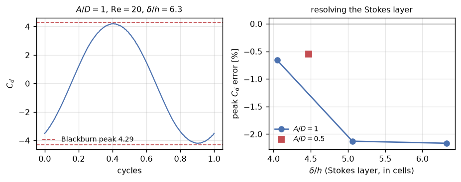
Results
| claim | measured | reference |
|---|---|---|
| spurious force, geometry static (the floor) | 6.97e-04 | — |
| spurious force, moving, seeding off | 3.07e-02 | 44x the floor |
| spurious force, moving, seeding on | 9.55e-04 | 1.4x the floor |
| drag bias vs the exact linearised answer, seeding off | +2.61% — and resolution-independent | 0 |
| drag bias, seeding on | -0.04% | 0 |
| refining \(\Delta t\) 4×, seeding off | 2.80e-02 -> 4.13e-02 | gets worse — spatial source |
| refining \(\Delta t\) 4×, seeding on | 3.07e-03 -> 6.26e-04 | converges to the floor |
| refining \(h\) 2×, seeding on | 1.56e-03 -> 8.16e-04 | floor 6.97e-04 |
| finite Re: peak \(C_d\), \(A/D=1\), Re\(=20\), \(\delta/h=6.3\) | 4.1971 | Blackburn (2002) 4.29 (-2.17%) |
| finite Re, \(A/D=0.5\), \(\delta/h=4.5\) | 5.6689 | Blackburn 5.70 (-0.54%, on the same \(\delta/h\) curve) |
| box sensitivity, \(L/D\) 7.5 → 10 | +0.11% | converged |
The headline is two numbers. A sphere that physically moves through the grid rings the drag at 44× the level of the same problem with a static interface, with a resolution-independent +2.6% bias on top — so yes, peclet.flow had the pathology the immersed-boundary literature describes, and no amount of grid or time-step refinement was going to remove the bias. Seeding the fresh cells with the local wall velocity brings both back to the non-moving floor, and with that in place — plus the advective wall-velocity fix described above — the finite-Reynolds-number peak drag sits within about two percent of Blackburn’s spectral value across the whole resolution ladder (2.17% at \(\delta/h = 6.3\)).
Adapt this yourself
- Change the motion.
set_instance_transformtakes any translation; a body on a prescribed path, a rotating one (quat), or a trajectory read from a DEM run all use the same call. - Turn the fix off with
set_fresh_cell_seed(False)and watch the ringing come back — that is how every number above was produced. - Push the amplitude. The spurious content grows with the number of cell crossings per cycle; at \(A/R = 1\) the sphere sweeps forty cells per cycle.
- Couple it.
peclet_coupling.ResolvedCfdDemdrives exactly this loop from apeclet.demparticle instead of a prescribed path.
Reproduce this
PECLET_LOCAL_BUILD=/path/to/suite/flow/build_l3_cuda \
  quarto render examples/moving-sphere-drag/index.qmd --execute
References
Blackburn, H. M. 2002. “Mass and Momentum Transport from a Sphere in Steady and Oscillatory Flows.” Physics of Fluids 14 (11): 3997–4011. https://doi.org/10.1063/1.1510448.
Lee, Jongho, Jungwoo Kim, Haecheon Choi, and Kyung-Soo Yang. 2011. “Sources of Spurious Force Oscillations from an Immersed Boundary Method for Moving-Body Problems.” Journal of Computational Physics 230 (7): 2677–95. https://doi.org/10.1016/j.jcp.2011.01.004.
Martins, Diogo M. C., Duarte M. S. Albuquerque, and José C. F. Pereira. 2017. “Continuity Constrained Least-Squares Interpolation for SFO Suppression in Immersed Boundary Methods.” Journal of Computational Physics 336: 608–26. https://doi.org/10.1016/j.jcp.2017.02.026.
Seo, Jung Hee, and Rajat Mittal. 2011. “A Sharp-Interface Immersed Boundary Method with Improved Mass Conservation and Reduced Spurious Pressure Oscillations.” Journal of Computational Physics 230 (19): 7347–63. https://doi.org/10.1016/j.jcp.2011.06.003.
Uhlmann, Markus. 2005. “An Immersed Boundary Method with Direct Forcing for the Simulation of Particulate Flows.” Journal of Computational Physics 209 (2): 448–76. https://doi.org/10.1016/j.jcp.2005.03.017.