import importlib.util, os, subprocess, sys
_local = os.environ.get("PECLET_LOCAL_BUILD")
if _local:
    sys.path.insert(0, _local)
elif importlib.util.find_spec("peclet") is None:
subprocess.run([sys.executable, "-m", "pip", "install", "-q", "peclet"], check=True)The Taylor–Green vortex: an exact Navier–Stokes solution
Advection injects divergence every step; the projection removes it, and the energy decays at exactly the viscous rate.
flow
projection
verification
unsteady
 Runs on a free Colab CPU runtime — the first cell installs
 peclet from PyPI.
What you’ll learn
How peclet handles unsteady incompressible flow with advection, and how to validate the pressure projection against a closed-form Navier–Stokes solution. The 2-D Taylor–Green vortex is one of the few exact solutions of the full nonlinear equations, so it is the standard test that (a) the projected velocity stays divergence-free even as advection tries to spoil it, and (b) the kinetic energy decays at exactly the analytic viscous rate.
The exact solution
In a triply-periodic box the incompressible Navier–Stokes equations admit
\[ u = U_0 \sin(kx)\cos(ky)\,e^{-2\nu k^2 t}, \quad v = -U_0 \cos(kx)\sin(ky)\,e^{-2\nu k^2 t}, \quad w = 0, \tag{1}\]
with \(k = 2\pi/L\). The nonlinear term is exactly balanced by a pressure gradient, and every Fourier mode decays as \(e^{-2\nu k^2 t}\) — so the domain-integrated kinetic energy decays as \(e^{-4\nu k^2 t}\). Advection is on, so each step the discrete convection injects a little divergence that the projection must remove.
import numpy as np
import matplotlib.pyplot as plt
from peclet import flow

plt.rcParams.update({"figure.dpi": 130, "font.size": 10, "axes.grid": True,
                     "grid.alpha": 0.3, "axes.axisbelow": True,
                     "figure.facecolor": "white", "savefig.bbox": "tight"})
BLUE, RED = "#1f77b4", "#d62728"
Initialising the exact field
The vortex is co-located at cell centres, so we use the collocated solver (flow.SolverColocated) and seed the exact \(t=0\) field with set_state. The box is triply periodic — no walls, no immersed solid (a trivial all-fluid SDF gives the full projection).
def tg_fields(N, nz, amp, U0=1.0):
    k = 2 * np.pi / N
    ix = np.arange(N)
    X, Y = np.meshgrid(ix, ix, indexing="ij")
    u = U0 * amp * np.sin(k * X) * np.cos(k * Y)
    v = -U0 * amp * np.cos(k * X) * np.sin(k * Y)
    rep = lambda a: np.asfortranarray(np.repeat(a[:, :, None], nz, axis=2))
    return rep(u), rep(v), np.asfortranarray(np.zeros((N, N, nz)))

def solve_tg(N, nz=4, nu=0.05, dt=0.5, steps=100, sample=5):
    k = 2 * np.pi / N
    s = flow.SolverColocated(N, N, nz)
    s.set_rho(1.0); s.set_mu(nu); s.set_dt(dt); s.set_advection(True)
    s.set_velocity_solver_params(80)
    s.set_solid(np.asfortranarray(np.ones((N, N, nz)) * 1e3), cutcell_pressure=True)
    u0, v0, w0 = tg_fields(N, nz, 1.0)
    s.set_state(u0, v0, w0)
    E0 = float(np.mean(u0 ** 2 + v0 ** 2))
    ts, E_meas = [0.0], [1.0]
    for it in range(steps):
        s.step()
        if (it + 1) % sample == 0:
            uu, vv = s.get_u(), s.get_v()
            ts.append((it + 1) * dt)
            E_meas.append(float(np.mean(uu ** 2 + vv ** 2)) / E0)
    T = dt * steps
    amp = np.exp(-2 * nu * k * k * T)
    ue, ve, we = tg_fields(N, nz, amp)
    uu, vv = s.get_u(), s.get_v()
    l2 = float(np.sqrt(np.mean((uu - ue) ** 2 + (vv - ve) ** 2)) / np.sqrt(E0))
    ts = np.array(ts)
    return dict(N=N, k=k, nu=nu, ts=ts, E_meas=np.array(E_meas),
                E_ana=np.exp(-4 * nu * k * k * ts), l2=l2,
                div=float(s.max_open_divergence()), u=s.get_u()[:, :, nz // 2],
                v=s.get_v()[:, :, nz // 2], u0=u0[:, :, nz // 2])

r = solve_tg(64)
print(f"N=64  final L2 error = {r['l2']:.3e}   max divergence = {r['div']:.1e}  (projection keeps it div-free)")
N=64 final L2 error = 7.893e-04 max divergence = 5.7e-16 (projection keeps it div-free)The vortex and its decay
u0f, v0f, _ = tg_fields(64, 1, 1.0)      # exact initial field
u2, v2 = u0f[:, :, 0], v0f[:, :, 0]
w0 = np.gradient(v2, axis=0) - np.gradient(u2, axis=1)   # vorticity

fig, (a0, a1) = plt.subplots(1, 2, figsize=(9, 3.9))
im = a0.imshow(w0.T, origin="lower", cmap="RdBu_r")
a0.set(title="vorticity, t=0", xlabel="x", ylabel="y"); a0.grid(False)
fig.colorbar(im, ax=a0, fraction=0.046, pad=0.04)

step = 6
xs = np.arange(0, 64, step)
X, Y = np.meshgrid(xs, xs, indexing="ij")
a1.quiver(X, Y, u2[::step, ::step], v2[::step, ::step])
a1.set(title="velocity field, t=0", xlabel="x", ylabel="y")
a1.set_aspect("equal"); a1.grid(False)
fig.tight_layout()
plt.show()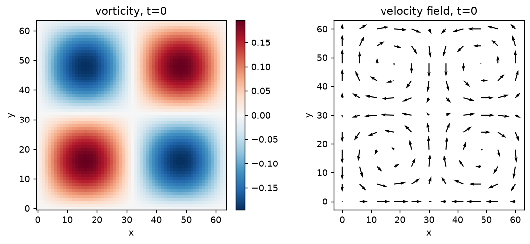
fig, ax = plt.subplots(figsize=(5.2, 3.8))
ax.plot(r["ts"], r["E_ana"], "-", color="0.15", lw=1.6, label=r"exact  $e^{-4\nu k^2 t}$")
ax.plot(r["ts"], r["E_meas"], "o", color=BLUE, ms=4, label="simulation (N=64)")
ax.set(xlabel="time", ylabel=r"kinetic energy  $E/E_0$", title="Taylor–Green viscous decay")
ax.legend()
plt.show()
print(f"energy error at final time = {abs(r['E_meas'][-1] - r['E_ana'][-1]):.2e}")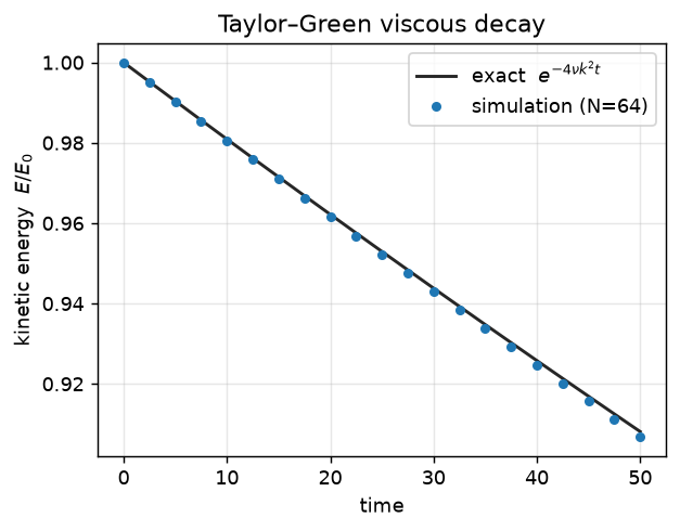
energy error at final time = 1.40e-03Convergence and divergence-freeness
Refining the grid drives the velocity error down, while the projected field stays divergence-free to solver tolerance at every resolution.
res = [solve_tg(N) for N in (32, 48, 64)]
Ns = np.array([d["N"] for d in res]); l2 = np.array([d["l2"] for d in res])
order = np.polyfit(np.log(Ns), np.log(l2), 1)[0]

fig, ax = plt.subplots(figsize=(5.0, 3.8))
ax.loglog(Ns, l2, "o-", color=RED, label="L2 error")
ax.loglog(Ns, l2[0] * (Ns / Ns[0]) ** -2.0, "k--", label=r"$\mathcal{O}(h^2)$")
ax.set(xlabel="N (box length in cells)", ylabel="L2 velocity error",
       title=f"Taylor–Green convergence — fitted order {order:.2f}")
ax.legend()
plt.show()
for d in res:
    print(f"  N={d['N']:3d}  L2={d['l2']:.3e}  max divergence={d['div']:.1e}")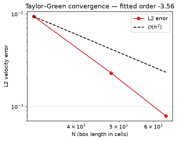
  N= 32  L2=9.366e-03  max divergence=4.0e-15
  N= 48  L2=2.301e-03  max divergence=5.3e-16
  N= 64  L2=7.893e-04  max divergence=5.7e-16
The error actually falls faster than the \(\mathcal{O}(h^2)\) reference: the Taylor–Green field is perfectly smooth and periodic, so the Koren TVD advection behaves like a higher-order scheme (no limiter clipping, no boundaries). The dashed line is a second-order floor, not the achieved rate — a nice reminder that formal order is a worst-case guarantee, and smooth problems often do better.
Adapt this yourself
- Change the Reynolds number. Lower
nufor a slower-decaying, more inertial vortex (watch the projection still hold the divergence to zero). - Run longer. Increase
steps— the energy should keep tracking the exponential all the way down. - 3-D Taylor–Green. Seed the classic 3-D initial condition instead and watch the enstrophy peak as vortices stretch — the canonical transition-to-turbulence test.
Reproduce this
pip install peclet
quarto render examples/taylor-green/index.qmd --execute
# ...or against a local source build:
PECLET_LOCAL_BUILD=/path/to/suite/flow/build_mpi OMP_NUM_THREADS=4 \
  quarto render examples/taylor-green/index.qmd --execute