# Makes this notebook run out-of-the-box on Colab/Binder. A real user just needs the
# published package; this installs it on first run. Authors can instead point at a
# local source build of the suite with the PECLET_LOCAL_BUILD env var.
import importlib.util, os, subprocess, sys
_local = os.environ.get("PECLET_LOCAL_BUILD")
if _local:
    sys.path.insert(0, _local)                                  # local source build
elif importlib.util.find_spec("peclet") is None:
subprocess.run([sys.executable, "-m", "pip", "install", "-q", "peclet"], check=True)Plane Poiseuille flow: the cut-cell IBM is exact on flat walls
Body-force channel flow past immersed no-slip walls — reproduced to machine precision.
flow
IBM
cut-cell
SDF
verification
 Runs on a free Colab CPU runtime — the first cell installs
 peclet from PyPI.
What you’ll learn
How to drive peclet’s incompressible flow solver, describe solid geometry with a signed distance function (SDF), and — the point of this example — how to correctly check the Robust-Scaled cut-cell immersed-boundary method against an analytic solution. The headline result: for flat immersed walls the method reproduces the exact velocity profile to solver tolerance at every resolution, because a second-order scheme is exact on a quadratic and a flat wall is represented exactly. (The cylindrical pipe shows what changes when the wall is curved.)
The problem
A constant body force \(F\) (force per unit volume, \(=-\mathrm{d}p/\mathrm{d}x\)) drives fluid down a channel of clear height \(H\) between two no-slip walls. The steady, fully developed profile is the parabola
\[ u(y) = \frac{F}{2\mu}\,(y-y_\text{lo})(y_\text{hi}-y), \qquad U_{\max} = \frac{F\,H^2}{8\mu}, \tag{1}\]
which is exactly quadratic in \(y\). A second-order discretization reproduces a quadratic with zero truncation error, so — provided the wall is represented exactly — the discrete solution should match Equation 1 at every grid node, at any resolution.
import numpy as np
import matplotlib.pyplot as plt
from peclet import flow

plt.rcParams.update({"figure.dpi": 130, "font.size": 10, "axes.grid": True,
                     "grid.alpha": 0.3, "axes.axisbelow": True,
                     "figure.facecolor": "white", "savefig.bbox": "tight"})
BLUE, RED, GREY = "#1f77b4", "#d62728", "0.80"
Geometry: two flat walls as an SDF
The SDF is negative inside the solid and positive in the fluid (peclet’s convention). For a slab of fluid between walls at \(y_\text{lo}\) and \(y_\text{hi}\), the signed distance to the nearer wall is min(y - ylo, yhi - y). Placing the walls at half-integer \(y\) puts them between grid nodes, so the wall cells are genuinely cut — this is not a lucky grid-aligned special case.
def channel_sdf(nx, ny, nz, ylo, yhi):
    """sdf[x,y,z] < 0 inside the solid walls, > 0 in the fluid slab (dx = 1)."""
    gy = np.arange(ny, dtype=np.float64)                 # velocity nodes at integer y
    sdf = np.empty((nx, ny, nz))
    sdf[:] = np.minimum(gy - ylo, yhi - gy)[None, :, None]
    return sdf

# Show the cut: walls at 5.5 / 11.5 leave fluid nodes y = 6..11, wall exactly between nodes.
sdf_demo = channel_sdf(8, 16, 8, 5.5, 11.5)
print("SDF along y (x,z fixed):", sdf_demo[4, :, 4])
SDF along y (x,z fixed): [-5.5 -4.5 -3.5 -2.5 -1.5 -0.5 0.5 1.5 2.5 2.5 1.5 0.5 -0.5 -1.5
-2.5 -3.5]Solve, and compare pointwise
We build a staggered-grid flow.Solver, set physical units, apply the body force and the SDF walls (cutcell_pressure=False — the flow is \(x\)-independent so the pressure projection is a no-op), and march to steady state with a large dt (backward Euler → steady Stokes).
The right way to validate is pointwise: compare the computed velocity at each fluid node to Equation 1 evaluated at the same node. (Comparing the discrete u.max() to the continuum peak \(U_\max\) is a trap — see the note below.)
def solve_channel(N, Solver=flow.Solver, F=0.01, mu=0.1, dt=50.0, max_steps=400):
    nx, nz = 8, 8
    ny = N
    ylo = round(0.30 * ny) + 0.5     # half-integer walls -> cut cells
    yhi = round(0.70 * ny) + 0.5
    H = yhi - ylo
    s = Solver(nx, ny, nz)
    s.set_rho(1.0); s.set_mu(mu); s.set_dt(dt)
    s.set_body_force(F, 0.0, 0.0)
    s.set_velocity_solver_params(200)
    s.set_pressure_solver_params(1)
    s.set_solid(channel_sdf(nx, ny, nz, ylo, yhi), cutcell_pressure=False)
    prev = 0.0
    for it in range(max_steps):
        s.step()
        u = s.get_u()
        if it > 5 and abs(float(u.max()) - prev) < 1e-10 * (abs(float(u.max())) + 1e-12):
            break
        prev = float(u.max())
    u = s.get_u()[nx // 2, :, nz // 2]
    gy = np.arange(ny, dtype=float)
    u_ana = np.where((gy > ylo) & (gy < yhi), (F / (2 * mu)) * (gy - ylo) * (yhi - gy), 0.0)
    fluid = (gy > ylo) & (gy < yhi)
    node_err = float(np.max(np.abs(u[fluid] - u_ana[fluid])))
    return dict(N=N, H=H, ylo=ylo, yhi=yhi, gy=gy, u=u, u_ana=u_ana, fluid=fluid,
                node_err=node_err, Umax_ana=F * H * H / (8 * mu))

r = solve_channel(32)
print(f"N=32  H={r['H']}  max|u_node - analytic_node| = {r['node_err']:.3e}   (machine/solver level)")
N=32 H=12.0 max|u_node - analytic_node| = 1.100e-06 (machine/solver level)The profile sits exactly on the parabola
yy = np.linspace(0, r["gy"][-1], 400)
ana_c = np.where((yy > r["ylo"]) & (yy < r["yhi"]),
                 (0.01 / (2 * 0.1)) * (yy - r["ylo"]) * (r["yhi"] - yy), np.nan)

fig, ax = plt.subplots(figsize=(4.6, 4.0))
ax.axhspan(r["gy"][0], r["ylo"], color=GREY, label="solid wall")
ax.axhspan(r["yhi"], r["gy"][-1], color=GREY)
ax.plot(ana_c, yy, "-", color="0.2", lw=1.5, label="analytic parabola")
ax.plot(r["u"][r["fluid"]], r["gy"][r["fluid"]], "o", color=BLUE, ms=6, label="cut-cell IBM (N=32)")
ax.set(xlabel="u(y)", ylabel="y", title="Plane Poiseuille through immersed walls")
ax.legend(loc="upper right", fontsize=8)
plt.show()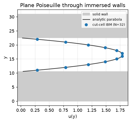
Exact at every resolution, on both meshes
peclet offers a staggered MAC grid (flow.Solver, the default) and a cell-centered/collocated grid (flow.SolverColocated). For flat walls both are exact — the pointwise node error stays at solver-tolerance level as the channel is refined (here refinement widens the channel at fixed spacing \(h=1\), so \(H\) grows).
print(f"{'N':>4} {'H':>5} {'staggered node err':>20} {'collocated node err':>21}")
for N in (16, 32, 64):
    rs = solve_channel(N, flow.Solver)
    rc = solve_channel(N, flow.SolverColocated)
    print(f"{N:4d} {rs['H']:5.1f} {rs['node_err']:20.3e} {rc['node_err']:21.3e}")
N H staggered node err collocated node err
16 6.0 6.493e-08 6.493e-08
32 12.0 1.100e-06 1.100e-06
64 26.0 2.468e-05 2.468e-05
ImportantA validation trap: never compare
u.max() to the continuum peak
It is tempting to check \(U_\max = F H^2/(8\mu)\) against u.max(). Don’t. The discrete maximum is sampled at a node, but with half-integer walls the channel centre falls on a half-integer — always \(0.5h\) from the nearest node. The parabola drops by \(\tfrac{F}{2\mu}(0.5h)^2\) over that half cell — a constant offset, independent of resolution — so u.max() sits a fixed amount below \(U_\max\), and dividing by \(U_\max\propto H^2\) manufactures a fake “converging” error sequence (2.8% → 0.7% → 0.15%). It looks like discretization error; it is pure sampling. Move the peak onto a node (keeping the walls cut) and u.max() matches \(U_\max\) to \(10^{-6}\). Always validate pointwise, node-to-node.
Adapt this yourself
- Change the geometry. Swap
channel_sdffor any SDF array (<0inside solid): a tilted channel, a wavy wall, a sphere packing. The cut-cell solver treats them all the same. - Curve the wall. A flat wall is represented exactly; a curved one is not — see the cylindrical pipe, where the same parabolic flow instead converges at second order.
- Go multi-rank. The identical script runs under
mpirun -np N python …;get_u()/get_p()are collective gathers returning the field on rank 0.
Reproduce this
The compiled solver runs this, so its outputs are frozen into the site. To regenerate:
pip install peclet            # the solver, from PyPI (CPU wheels run this example)
quarto render examples/poiseuille-ibm/index.qmd --execute
# ...or against a local source build of the suite (no wheel needed):
PECLET_LOCAL_BUILD=/path/to/suite/flow/build_mpi OMP_NUM_THREADS=4 \
  quarto render examples/poiseuille-ibm/index.qmd --execute