import importlib.util, os, subprocess, sys
_local = os.environ.get("PECLET_LOCAL_BUILD")
if _local:
    for p in _local.split(os.pathsep):
        sys.path.insert(0, p)
elif importlib.util.find_spec("peclet") is None:
subprocess.run([sys.executable, "-m", "pip", "install", "-q", "peclet"], check=True)3-D Rayleigh–Bénard convection on the GPU
Heat a box of air from below until it overturns: a transported temperature field, Boussinesq buoyancy, the critical Rayleigh number of 1708, and turbulent heat transport matched to published DNS — all on the GPU.
flow
scalar-transport
boussinesq
natural-convection
benchmark
gpu
visualization
 The onset study runs anywhere (a few minutes on GPU); the turbulent-cube sections want a CUDA build — on a free Colab CPU runtime shrink the grids as noted inline.
What you’ll learn
How to turn the single-phase solver into a thermal convection code with two calls: add_scalar("T", …) registers temperature as a transported scalar (advection–diffusion on the same cut-cell grid), and set_property_model("force_z", "boussinesq", "T", …) closes the loop by writing the buoyancy body force from that field every step — the Boussinesq approximation. We then validate the coupled physics twice, against the two classic yardsticks of Rayleigh–Bénard convection:
- The onset. Between rigid plates, convection starts at the critical Rayleigh number \(\mathrm{Ra}_c = 1707.76\) — a number derived by linear stability theory (Chandrasekhar 1961). We measure exponential growth/decay rates of a tiny perturbation on both sides of the threshold and bracket \(\mathrm{Ra}_c\) to a fraction of a percent.
- Turbulent heat transport. In a cubical cell at \(\mathrm{Ra} = 10^6\) and \(3\times10^6\) (\(\mathrm{Pr}=0.7\)) we time-average the Nusselt number and compare with the lattice-Boltzmann DNS of Xu et al. (2019) (and the classic \(\mathrm{Nu}\sim\mathrm{Ra}^{2/7}\) scaling of hard turbulence, Kerr (1996)).
And because a convecting box is one of the prettiest objects in fluid dynamics, we render the plumes in 3-D and film them.
The physics
Under the Boussinesq approximation the fluid is incompressible with constant properties, except that density variations with temperature survive in the gravity term — a linear expansion \(\rho \approx \rho_0(1 - \beta(T - T_0))\) turns into a buoyancy body force:
\[ \partial_t \mathbf{u} + (\mathbf{u}\cdot\nabla)\mathbf{u} = -\tfrac{1}{\rho_0}\nabla p + \nu \nabla^2 \mathbf{u} + g\beta\,(T - T_0)\,\hat{\mathbf{z}}, \qquad \nabla\cdot\mathbf{u}=0 \tag{1}\]
\[ \partial_t T + \nabla\cdot(\mathbf{u} T) = \alpha \nabla^2 T \tag{2}\]
Two dimensionless groups govern everything: the Rayleigh number \(\mathrm{Ra} = g\beta\,\Delta T\, H^3/(\nu\alpha)\) (buoyancy forcing over diffusion) and the Prandtl number \(\mathrm{Pr} = \nu/\alpha\) (momentum over heat diffusivity; air is \(\mathrm{Pr}\simeq0.7\)). The answer of the system is the Nusselt number — the heat flux through the layer over the flux pure conduction would carry:
\[ \mathrm{Nu} \;=\; \frac{\langle w T\rangle - \alpha\,\partial_z \langle T\rangle} {\alpha\,\Delta T / H}. \tag{3}\]
The solver works in grid units (\(\Delta x = 1\), so \(H = N\) cells, and we set \(\Delta T = 1\)). We choose the free-fall velocity \(u_f = \sqrt{g\beta\,\Delta T\,H}\) — the natural velocity scale of convection — to be a CFL-friendly value, and derive the transport coefficients from \(\mathrm{Ra}\) and \(\mathrm{Pr}\):
\[ g\beta = u_f^2/H, \qquad \nu = u_f H \sqrt{\mathrm{Pr}/\mathrm{Ra}}, \qquad \alpha = \nu/\mathrm{Pr}. \tag{4}\]
One free-fall time \(t_f = H/u_f\) is then \(H/u_f\) steps at \(\mathrm{d}t=1\).
import numpy as np
import time
import matplotlib.pyplot as plt
from peclet import flow

plt.rcParams.update({"figure.dpi": 130, "font.size": 10, "axes.grid": True,
                     "grid.alpha": 0.3, "axes.axisbelow": True,
                     "figure.facecolor": "white", "savefig.bbox": "tight"})
BLUE, RED, GREEN = "#1f77b4", "#d62728", "#2ca02c"
print("backend:", flow.execution_space)
backend: CudaThe whole thermal setup is one function. Temperature is registered as a transported scalar (advected by the just-projected velocity with a Koren-TVD flux, diffused implicitly), given Dirichlet values on the hot floor and cold ceiling and adiabatic (zero-flux) or periodic sides, and coupled back into the momentum equation through the boussinesq property closure, which fills the per-cell body force force_z \(= \rho_0 g\beta\,(T - T_0)\) at the top of every step.
def rb_solver(nx, ny, N, Ra, Pr=0.7, u_f=0.4, sides="adiabatic", dt=1.0,
              vel_iters=12, scal_iters=8, pcg=(60, 1e-2)):
    """A Rayleigh-Benard box: hot floor (T=1), cold ceiling (T=0), gravity in -z.
    sides: 'adiabatic' no-slip walls, or 'periodic'. Grid units: dx=1, H=N, dT=1."""
    nu = u_f * N * np.sqrt(Pr / Ra)          # from Ra, Pr at the chosen u_f  (@eq-units)
    alpha = nu / Pr
    gbeta = u_f ** 2 / N
    s = flow.Solver(nx, ny, N)
    s.set_rho(1.0); s.set_mu(nu); s.set_dt(dt)
    s.set_advection(True)                     # explicit Koren-TVD momentum advection
    s.set_velocity_solver_params(vel_iters)   # diffusion number nu*dt ~ 0.04 -> converges fast
    s.set_pressure_multigrid(True, 6)
    s.set_pressure_pcg(True, *pcg); s.set_pressure_warmstart(True)
    s.set_domain_bc(4, 1); s.set_domain_bc(5, 1)          # rigid floor + ceiling
    if sides == "adiabatic":
        for f in (0, 1, 2, 3):
            s.set_domain_bc(f, 1)                         # no-slip side walls
    s.set_pressure_geometry(np.asfortranarray(np.full((nx, ny, N), 1e30)))  # all fluid
    s.add_scalar("T", diffusivity=alpha, scheme=1, iters=scal_iters)
    s.set_scalar_bc("T", 4, 2, 1.0)                       # floor   T = 1 (Dirichlet)
    s.set_scalar_bc("T", 5, 2, 0.0)                       # ceiling T = 0
    if sides == "adiabatic":
        for f in (0, 1, 2, 3):
            s.set_scalar_bc("T", f, 1)                    # zero-flux sides
    # the Boussinesq closure: force_z = rho0 * gbeta * (T - T0), refreshed every step
    s.set_property_model("force_z", "boussinesq", "T", [1.0, gbeta, 1.0, 0.5])
    return s, nu, alpha


def linear_profile(nx, ny, N):
    z = (np.arange(N) + 0.5) / N
    return np.zeros((nx, ny, N)) + (1.0 - z)[None, None, :]


def nusselt(s, N, alpha):
    """Three independent Nu estimates: hot-wall / cold-wall gradient + volume average."""
    T = s.get_field("T")
    w = s.get_w()                              # staggered: w[...,k] is the -z face of cell k
    wc = 0.5 * (w + np.roll(w, -1, 2))         # cell centres (both boundary faces are 0)
    Nu_bot = 2.0 * N * (1.0 - T[:, :, 0].mean())    # ghost = 2*Tw - T  ->  half-cell gradient
    Nu_top = 2.0 * N * T[:, :, -1].mean()
    Nu_vol = 1.0 + (wc * (T - 0.5)).mean() * N / alpha    # @eq-nu, volume-averaged
    return Nu_bot, Nu_top, Nu_vol
Part 1 — the onset: measuring \(\mathrm{Ra}_c\)
Below a critical Rayleigh number, the conductive state (fluid at rest, linear temperature profile) is stable: every disturbance dies. Above it, buoyancy beats diffusion and convection rolls grow exponentially. For rigid-rigid plates linear stability theory gives \(\mathrm{Ra}_c = 1707.762\) at critical wavenumber \(a_c = 3.117\) (Chandrasekhar 1961) — one of the sharpest quantitative predictions in fluid dynamics, and a merciless test of the coupled solver: get any factor in the buoyancy–advection–diffusion loop slightly wrong and the threshold moves.
We use a laterally periodic box of width \(2H\), whose gravest mode has wavelength \(2H\) — i.e. wavenumber \(2\pi H/2H = \pi \approx a_c\), so the marginal Rayleigh number of the box is within 0.03% of the true minimum. We seed the conductive profile with a tiny thermal perturbation and fit the exponential rate \(\sigma\) of the vertical-velocity norm on both sides of the threshold. The zero crossing of \(\sigma(\mathrm{Ra})\) is our measured \(\mathrm{Ra}_c\).
def growth_rate(Ra, N=32, steps=2500, dt=2.0, sample=25):
    # near onset the velocities are ~1e-5: CFL is no constraint, so pick u_f large to
    # shorten the diffusive clock (u_f=1.5 -> nu~1, ~7 diffusion times in 2500 steps);
    # and the PCG's relative stopping test never fires on a near-quiescent field, so
    # cap it at 12 iterations -> a fixed-work MG solve (divergence stays ~1e-12 here)
    s, nu, alpha = rb_solver(2 * N, 2 * N, N, Ra, sides="periodic", dt=dt, u_f=1.5,
                             vel_iters=60, scal_iters=30, pcg=(12, 1e-6))
    x = (np.arange(2 * N) + 0.5) / (2 * N)
    z = (np.arange(N) + 0.5) / N
    T0 = linear_profile(2 * N, 2 * N, N)
    T0 += 1e-4 * np.sin(2 * np.pi * x)[:, None, None] * np.sin(np.pi * z)[None, None, :]
    s.set_field("T", np.asfortranarray(T0))
    ts, amps = [], []
    for it in range(steps):
        s.step()
        if it % sample == sample - 1:
            w = s.get_w()
            ts.append((it + 1) * dt); amps.append(float(np.sqrt((w * w).mean())))
    del s
    t_kappa = N * N / alpha                   # vertical diffusion time (grid units)
    ts, amps = np.array(ts) / t_kappa, np.array(amps)
    m = len(ts) // 2                          # fit past the initial transient
    sig = np.polyfit(ts[m:], np.log(amps[m:]), 1)[0]   # growth rate in 1/t_kappa
    return sig, ts, amps


# keep the sweep close to the threshold: much beyond ~1.1 Ra_c the mode saturates
# nonlinearly inside the run and the late-time fit under-reports the linear rate
RAS = [1500, 1600, 1700, 1750, 1850]
curves, sigmas = {}, []
for Ra in RAS:
    sig, ts, amps = growth_rate(Ra)
    curves[Ra] = (ts, amps); sigmas.append(sig)
    print(f"Ra={Ra}:  sigma = {sig:+.4f} / t_kappa", flush=True)

c = np.polyfit(RAS, sigmas, 1)
Ra_c = -c[1] / c[0]
err = abs(Ra_c - 1707.762) / 1707.762 * 100
print(f"\nmeasured Ra_c = {Ra_c:.0f}    (linear stability theory: 1707.76 -> {err:.2f}% off)")
Ra=1500: sigma = -1.3108 / t_kappa
Ra=1600: sigma = -0.6458 / t_kappa
Ra=1700: sigma = +0.0032 / t_kappa
Ra=1750: sigma = +0.3218 / t_kappa
Ra=1850: sigma = +0.9449 / t_kappa
measured Ra_c = 1701 (linear stability theory: 1707.76 -> 0.38% off)fig, (a0, a1) = plt.subplots(1, 2, figsize=(9, 3.6))
shades = plt.cm.viridis(np.linspace(0.05, 0.85, len(RAS)))
for c, (Ra, (ts, amps)) in zip(shades, curves.items()):
a0.semilogy(ts, amps, lw=1.5, color=c, label=f"Ra={Ra}")
a0.set(xlabel=r"$t/t_\kappa$", ylabel=r"$\Vert w\Vert_2$")
a0.legend(fontsize=7, ncol=2)
a1.plot(RAS, sigmas, "o-", color=BLUE, label=r"measured $\sigma$")
a1.axhline(0.0, color="0.6", lw=0.8)
a1.axvline(1707.762, ls="--", color=RED, label=r"$\mathrm{Ra}_c$ = 1707.76 (theory)")
a1.axvline(Ra_c, ls=":", color=BLUE, label=f"zero crossing = {Ra_c:.0f}")
a1.set(xlabel="Ra", ylabel=r"$\sigma \cdot t_\kappa$")
a1.legend(fontsize=8)
fig.tight_layout(); plt.show()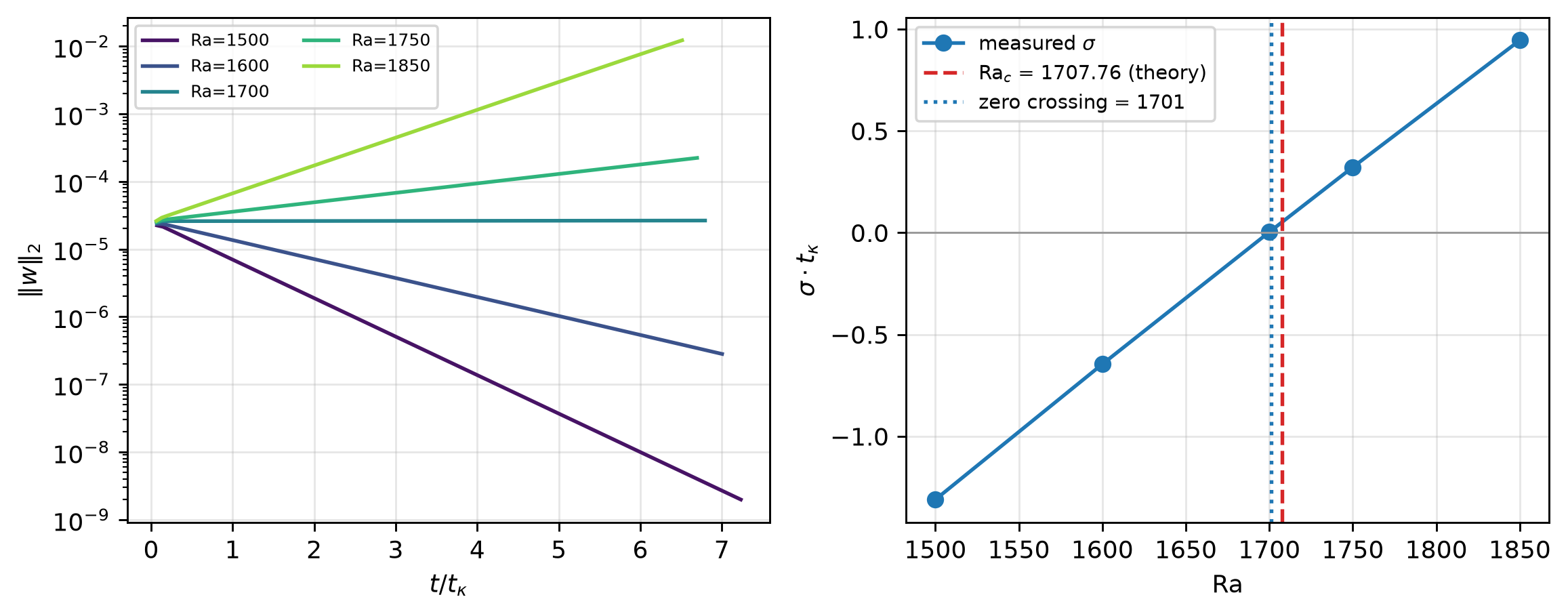
Part 2 — turbulent convection in a cube
Push \(\mathrm{Ra}\) four orders of magnitude past the onset and the neat rolls give way to a turbulent dance of thermal plumes. The heat transport becomes the quantitative question: how much does convection multiply the conductive flux? For a cubical cell with adiabatic sidewalls at \(\mathrm{Pr}=0.7\), Xu et al. (2019) tabulate DNS values (their Table 4): \(\mathrm{Nu} = 8.34\) at \(\mathrm{Ra}=10^6\) and \(\mathrm{Nu} = 11.47\) at \(3\times10^6\), following the hard-turbulence scaling \(\mathrm{Nu} = 0.153\,\mathrm{Ra}^{0.289}\) (cf. the \(\mathrm{Ra}^{2/7}\) of Kerr (1996)).
We run the same cell — no-slip everywhere, hot floor, cold ceiling, adiabatic sides — and time-average three independent Nusselt estimates (hot-wall gradient, cold-wall gradient, volume average of \(wT\)): their mutual agreement is a resolution check.
def run_cube(N, Ra, spin_tf, avg_tf, seed=11, movie_every=0, movie_tf=0):
    s, nu, alpha = rb_solver(N, N, N, Ra)
    tf = int(N / 0.4)                          # steps per free-fall time
    T0 = linear_profile(N, N, N)
    x = (np.arange(N) + 0.5) / N
    z = (np.arange(N) + 0.5) / N
    T0 += 0.3 * (np.sin(np.pi * x)[:, None, None] - 0.5) * np.sin(np.pi * z)[None, None, :]
    T0 += 0.02 * np.random.default_rng(seed).standard_normal(T0.shape)
    s.set_field("T", np.asfortranarray(T0))
    t0 = time.time()
    for it in range(spin_tf * tf):             # spin-up (discarded)
        s.step()
    series = []
    for it in range(avg_tf * tf):              # averaging window
        s.step()
        if it % (tf // 4) == tf // 4 - 1:
            series.append(nusselt(s, N, alpha))
    frames = []
    for it in range(movie_tf * tf):            # optional: keep stepping, film it
        s.step()
        if it % movie_every == movie_every - 1:
            frames.append(np.asarray(s.get_field("T"), dtype=np.float32))
    T, w = s.get_field("T"), s.get_w()
    wall = time.time() - t0
    print(f"N={N} Ra={Ra:.0e}: {(spin_tf+avg_tf)*tf} steps in {wall/60:.0f} min "
          f"({wall/((spin_tf+avg_tf+movie_tf)*tf)*1e3:.0f} ms/step)", flush=True)
    del s
    return np.array(series), T, w, frames


res = {}
res[1e6] = run_cube(128, 1e6, spin_tf=200, avg_tf=300, movie_every=128, movie_tf=50)
res[3e6] = run_cube(144, 3e6, spin_tf=150, avg_tf=250)
N=128 Ra=1e+06: 160000 steps in 114 min (39 ms/step)
N=144 Ra=3e+06: 144000 steps in 133 min (55 ms/step)XU = {1e6: 8.34, 3e6: 11.47} # Xu, Shi & Xi (2019), Table 4 (Nu_vol/Nu_wall mean)
rows = []
for Ra, (series, *_rest) in res.items():
nu_mean = series.mean(0) # [bot, top, vol]
nb = 6
blocks = series[: len(series) // nb * nb, 0].reshape(nb, -1).mean(1)
err = blocks.std(ddof=1) / np.sqrt(nb)
rows.append((Ra, *nu_mean, err, XU[Ra]))
print(f"Ra={Ra:.0e}: Nu_bot={nu_mean[0]:.2f} Nu_top={nu_mean[1]:.2f} "
f"Nu_vol={nu_mean[2]:.2f} (+-{err:.2f}) Xu et al.: {XU[Ra]}", flush=True)Ra=1e+06: Nu_bot=8.32 Nu_top=8.32 Nu_vol=8.31 (+-0.08) Xu et al.: 8.34
Ra=3e+06: Nu_bot=11.39 Nu_top=11.39 Nu_vol=11.38 (+-0.09) Xu et al.: 11.47fig, (a0, a1) = plt.subplots(1, 2, figsize=(9.2, 3.6))
series = res[1e6][0]
tt = np.arange(len(series)) * 0.25
a0.plot(tt, series[:, 0], lw=0.8, color=BLUE, label=r"$\mathrm{Nu}_\mathrm{bot}(t)$")
a0.plot(tt, series[:, 2], lw=0.8, color=GREEN, alpha=0.7, label=r"$\mathrm{Nu}_\mathrm{vol}(t)$")
a0.axhline(XU[1e6], ls="--", color=RED, label="Xu et al. 2019")
a0.set(xlabel=r"$t/t_f$", ylabel="Nu", title=r"$\mathrm{Ra}=10^6$")
a0.legend(fontsize=8)
raa = np.logspace(5.7, 7.2, 50)
a1.loglog(raa, 0.153 * raa ** 0.289, "--", color=RED, lw=1.2,
label=r"$0.153\,\mathrm{Ra}^{0.289}$ (Xu et al. fit)")
for (Ra, nb_, nt_, nv_, err, xu) in rows:
a1.errorbar([Ra], [(nb_ + nt_ + nv_) / 3], yerr=[err], fmt="o", color=BLUE,
ms=6, capsize=4)
a1.plot([Ra], [xu], "s", color="0.15", ms=6)
a1.plot([], [], "o", color=BLUE, label="peclet (this notebook)")
a1.plot([], [], "s", color="0.15", label="Xu et al. 2019 (DNS)")
a1.set(xlabel="Ra", ylabel="Nu")
a1.legend(fontsize=8)
fig.tight_layout(); plt.show()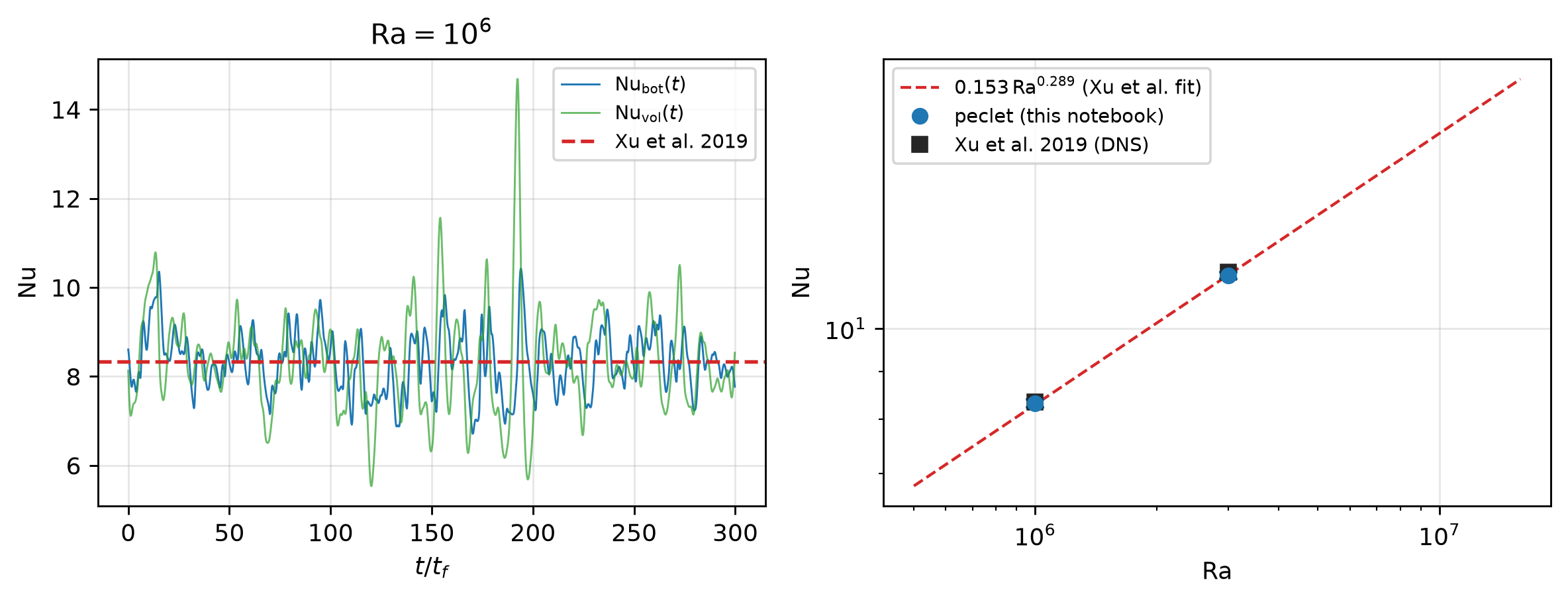
The plumes, in 3-D
The classic visual of Rayleigh–Bénard convection: sheets of hot fluid peel off the floor, organize into mushroom plumes, and crash into the ceiling (and vice versa, cold plumes raining down). We render the \(\mathrm{Ra}=3\times10^6\) final snapshot — isosurfaces of temperature slightly above/below the mean, over a mid-plane slice.
import pyvista as pv
pv.OFF_SCREEN = True

T3 = res[3e6][1]
N3 = T3.shape[0]
grid = pv.ImageData(dimensions=T3.shape, spacing=(1 / N3,) * 3)
grid["T"] = T3.flatten(order="F")
hot = grid.contour([0.6], scalars="T")
cold = grid.contour([0.4], scalars="T")
slc = grid.slice(normal="y", origin=(0.5, 0.5, 0.5))

pl = pv.Plotter(off_screen=True, window_size=(1100, 900))
pl.background_color = "white"
pl.add_mesh(slc, cmap="coolwarm", clim=(0.2, 0.8), show_scalar_bar=False, opacity=0.9)
pl.add_mesh(hot, color="#c0392b", smooth_shading=True, specular=0.4, opacity=0.95)
pl.add_mesh(cold, color="#2c5aa0", smooth_shading=True, specular=0.4, opacity=0.95)
pl.add_mesh(grid.outline(), color="#4d4d4d", line_width=1.2)
pl.camera_position = [(2.4, -1.6, 1.7), (0.5, 0.5, 0.45), (0, 0, 1)]
img = pl.screenshot(return_img=True); pl.close()
figp, axp = plt.subplots(figsize=(7.2, 6))
axp.imshow(img); axp.axis("off"); plt.show()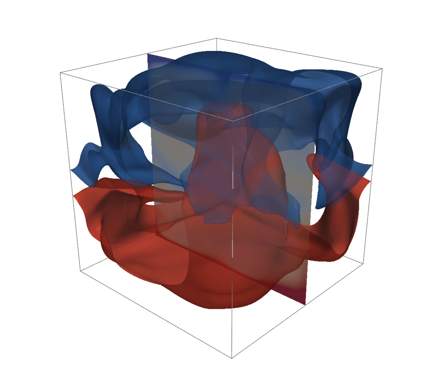
And the movie — 50 free-fall times of the \(\mathrm{Ra}=10^6\) cell, one frame per 0.4 \(t_f\):
import imageio.v2 as imageio

frames = res[1e6][3]
writer = imageio.get_writer("rayleigh_benard.mp4", fps=16, quality=8)
for Tf in frames:
    g = pv.ImageData(dimensions=Tf.shape, spacing=(1 / Tf.shape[0],) * 3)
    g["T"] = Tf.flatten(order="F")
    pl = pv.Plotter(off_screen=True, window_size=(768, 624))
    pl.background_color = "white"
    pl.add_mesh(g.slice(normal="y", origin=(0.5, 0.5, 0.5)), cmap="coolwarm",
                clim=(0.2, 0.8), show_scalar_bar=False, opacity=0.9)
    pl.add_mesh(g.contour([0.6], scalars="T"), color="#c0392b", smooth_shading=True)
    pl.add_mesh(g.contour([0.4], scalars="T"), color="#2c5aa0", smooth_shading=True)
    pl.add_mesh(g.outline(), color="#4d4d4d", line_width=1.2)
    pl.camera_position = [(2.4, -1.6, 1.7), (0.5, 0.5, 0.45), (0, 0, 1)]
    writer.append_data(pl.screenshot(return_img=True)); pl.close()
writer.close()
print(f"{len(frames)} frames -> rayleigh_benard.mp4")
125 frames -> rayleigh_benard.mp4Adapt this yourself
- Water instead of air.
Pr=7: the plumes get thinner and the flow smoother at the same \(\mathrm{Ra}\) — Xu et al. (2019) tabulate that case too (\(\mathrm{Nu}=8.49\) at \(10^6\)), so the comparison extends directly. - Wider boxes. Replace the cube by
rb_solver(4*N, 4*N, N, ..., sides="periodic")for a slab: the large-scale circulation disappears into a pattern of plume clusters. - Temperature-dependent viscosity. Swap the constant
mufor an Arrhenius closure (set_property_model("mu", "arrhenius", "T", [...])) — the same closure seam that carried the buoyancy. - Immersed obstacles. Everything here composes with
set_solid: drop an SDF sphere array into the cell and you have convection in a porous layer (the immersed solid is adiabatic by construction — closed faces carry no flux).
Reproduce this
pip install peclet    # CPU wheels; for CUDA: pip install peclet-flow-cu13
quarto render examples/rayleigh-benard/index.qmd --execute
# ...or against a local source build (GPU):
PECLET_LOCAL_BUILD=/path/to/suite/flow/build_cuda \
  quarto render examples/rayleigh-benard/index.qmd --execute
The production numbers in this page were produced on a single RTX 5080 (peclet.flow Kokkos/CUDA backend): 36 ms per step on the \(128^3\) cube — the full page (onset sweep + two turbulent cubes + movie) renders in ~4–5 hours.
References
Chandrasekhar, Subrahmanyan. 1961. Hydrodynamic and Hydromagnetic Stability. Clarendon Press.
Kerr, Robert M. 1996. “Rayleigh Number Scaling in Numerical Convection.” Journal of Fluid Mechanics 310: 139–79. https://doi.org/10.1017/S0022112096001760.
Xu, Ao, Le Shi, and Heng-Dong Xi. 2019. “Lattice Boltzmann Simulations of Three-Dimensional Thermal Convective Flows at High Rayleigh Number.” International Journal of Heat and Mass Transfer 140: 359–70. https://doi.org/10.1016/j.ijheatmasstransfer.2019.06.002.