Wall-bounded turbulence: channel-flow DNS vs Moser–Kim–Mansour
Direct numerical simulation of turbulent plane-channel flow that reproduces the classic Moser–Kim–Mansour 1999 DNS — mean-velocity profile on the log law, fluctuation peaks on the reference, friction velocity exact — from a 182 M-cell run on 4 × H100 of the Snellius supercomputer.
What you’ll learn
How to run a direct numerical simulation (DNS) of turbulent plane-channel flow with the peclet.flow solver — the canonical wall-bounded-turbulence testbed — and validate it against the reference database of Moser, Kim & Mansour (Moser et al. (1999)) at \(Re_\tau = 180\): the mean-velocity profile, the Reynolds stresses, and the friction velocity, all in wall units. You’ll see how the channel is driven (constant pressure gradient vs constant flow rate), how the statistics are gathered, why matching MKM quantitatively is a resolution question, and how to run the full-resolution DNS efficiently on the Snellius supercomputer (multi-GPU, GPU-aware MPI, checkpoint/restart job scripts). The multi-GPU performance — a measured weak-scaling study — is split into a companion scaling benchmark.
This example is also honest about a solver limitation and turns it into the physics lesson: peclet.flow uses upwind advection on an isotropic grid, so on a coarse grid numerical dissipation damps the turbulence — and the cure is resolution, which is exactly what motivates going to HPC.
The problem
Plane channel flow: incompressible flow between two parallel no-slip walls, periodic in the streamwise (\(x\)) and spanwise (\(z\)) directions, driven by a uniform body force \(f\) that stands in for a mean pressure gradient. With half-height \(H\) and kinematic viscosity \(\nu\), the friction velocity \(u_\tau=\sqrt{\tau_w/\rho}\) and the friction Reynolds number \(Re_\tau = u_\tau H/\nu\) organise everything. The benchmark case is \(Re_\tau=180\).
A global momentum balance makes the driving trivial: at a statistically steady state the wall shear must balance the body force, \(\tau_w = f H\), so constant-pressure-gradient (CPG) forcing pins \(u_\tau=\sqrt{fH/\rho}\) exactly. We work in grid units (\(\Delta x=\Delta y=\Delta z=1\)) and choose \(u_\tau=1\), so every statistic comes out directly in wall units: \(u^+=u\), \(y^+=y/\nu\), and
\[ \nu = \frac{H}{Re_\tau}, \qquad f = \frac{\rho\,u_\tau^2}{H} = \frac{2}{n_y}, \qquad \Delta^+ = \frac{u_\tau\,\Delta}{\nu} = \frac{360}{n_y}. \tag{1}\]
The last identity is the crux for this solver: the grid is isotropic (no wall-normal stretching), so the spacing in wall units is the same in every direction, \(\Delta^+ = 360/n_y\). A spectral channel DNS clusters points near the wall (MKM used \(128\times129\times128\) with Chebyshev stretching); here every cell is a cube, which is simpler but means the wall-parallel directions are over-resolved and the total cell count grows as \(n_y^3\).
The setup in code
The whole driver is channel_dns.py (single-GPU) and channel_dns_mpi.py (distributed). The core is a dozen calls:
from peclet import flow
import numpy as np

nx, ny, nz = 384, 128, 128            # reduced box Lx=6H, Lz=2H ; Delta+ = 360/ny = 2.8
nu = (ny/2)/180.0                     # Re_tau = 180
s = flow.Solver(nx, ny, nz)           # staggered MAC, exact projection
s.set_rho(1.0); s.set_mu(nu); s.set_dt(0.012)
s.set_advection(True); s.set_advection_scheme(0)          # 0 = 2nd-order upwind (least dissipative)
s.set_pressure_multigrid(True, 5); s.set_pressure_pcg(True, 80, 1e-4); s.set_pressure_warmstart(True)
s.set_domain_bc(2, 1); s.set_domain_bc(3, 1)              # no-slip walls on -y,+y ; x,z periodic
s.set_body_force(2.0/ny, 0.0, 0.0)                        # CPG: pins u_tau = 1
s.set_pressure_geometry(np.full((nx, ny, nz), 1e30, order='F'))   # all-fluid (domain-BC path)
s.set_state(u0, v0, w0)               # turbulent initial guess (Reichardt mean + near-wall noise)
for it in range(nsteps):
    s.step()
Getting a channel to become turbulent at \(Re_\tau=180\) — a fragile low-Reynolds point — needs more than random noise: the initial field seeds streamwise rolls and streaks at the streak spanwise wavelength (~110 wall units), the coherent structures that drive the self-sustaining turbulence cycle, with all perturbation scales set in wall units (resolution-independent). Statistics (\(\langle U\rangle\), \(\langle u'^2\rangle\), \(\langle u'v'\rangle\), …) are then averaged over the homogeneous \(x,z\) planes and over time, folded about the centreline.
CPG (set_body_force) pins \(u_\tau=1\) exactly (so \(Re_\tau=180\) by construction) — the robust drive for reaching and sustaining turbulence, and a laminarizing flow is obvious (the bulk \(U_b^+\) climbs instead of holding ~15.7). Constant flow rate (CFR) holds \(U_b^+\) fixed (on-device via CuPy) and reads the emergent friction from momentum balance, \(u_\tau^2 = H\langle\delta\rangle/\Delta t\) — useful once the flow is turbulent, but it will happily hold a laminar flux too, so it is not the choice for transition. The production scripts default to CPG; both are in the driver.
Validated against MKM 1999
At the production resolution — the full MKM box at \(\Delta^+=1.5\) (182 M cells, 4 × H100 on Snellius), CPG forcing so \(Re_\tau=180\) exactly, time-averaged over ~7 eddy-turnovers — peclet.flow reproduces the Moser–Kim–Mansour statistics quantitatively:
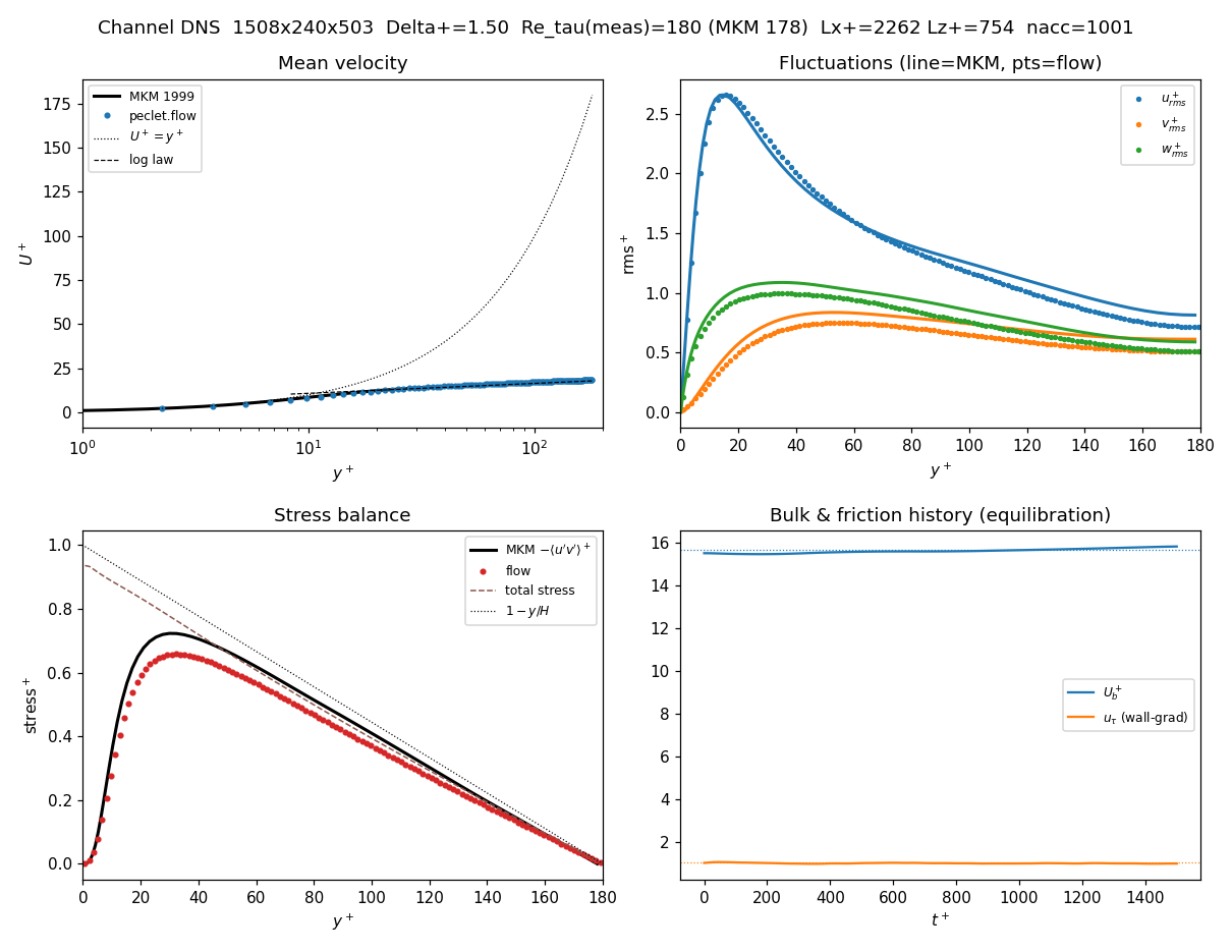
peclet.flow, lines are MKM. Mean velocity on the log law; streamwise/spanwise rms peaks on the reference; total stress closing the \(1-y/H\) balance; and the bulk/friction history confirming a sustained, equilibrated turbulent state.| quantity | \(\Delta^+=2.8\) (coarse, 1 GPU) | \(\Delta^+=1.5\) (production, 4 GPU) | MKM 1999 |
|---|---|---|---|
| centreline \(U^+\) | 24.4 | 18.2 | 18.3 |
| log law \(\kappa\), \(B\) | — | 0.39, 5.2 | 0.41, 5.2 |
| \(u_{rms}^+\) peak | 2.36 | 2.66 | 2.66 |
| \(w_{rms}^+\) peak | — | 0.99 | ~1.0 |
| \(-\langle u'v'\rangle^+\) peak | 0.43 | 0.658 | 0.72 |
The mean profile lands on the log law (centreline within 0.4 %; \(\kappa,B\) matching), the streamwise and spanwise fluctuation peaks are on MKM, and the resolved plus viscous stress closes the linear \(1-y/H\) balance. The one quantity still ~9 % low is the Reynolds shear-stress peak — the expected signature of the isotropic grid: with no near-wall clustering, \(\Delta y^+=1.5\) at the wall is much coarser than MKM’s stretched \(\Delta y^+\approx0.05\), so the peak-producing near-wall motions are slightly under-resolved (the fine/hero presets below push \(\Delta y^+\) down further).
The resolution ladder is the validation. The coarse \(\Delta^+=2.8\) single-GPU run sits well short of MKM (\(Re_\tau=142\), damped outer layer, \(-\langle u'v'\rangle\) at 59 %) because the second-order upwind advection acts like an eddy viscosity; halving \(\Delta^+\) to 1.5 removes almost all of that gap. That monotone approach to the reference as \(\Delta^+\) drops — the model converging as the numerical dissipation is resolved away — is exactly what a benchmark should show. The full-resolution run that gets there is a supercomputer-scale job; the rest of this page is how to run it.
The production benchmark run on Snellius
A DNS in the full MKM box \(4\pi H\times 2H\times \tfrac{4}{3}\pi H\) at a resolution that beats the numerical dissipation is multi-GPU work. On the isotropic grid the cell count is \(\approx 13.2\,n_y^3\), and finer \(\Delta^+\) (larger \(n_y\)) means less numerical dissipation → closer to MKM:
| resolution | \(\Delta^+\) | grid \(n_x\times n_y\times n_z\) | cells | H100s (nodes) |
|---|---|---|---|---|
| production | 1.5 | \(1508\times240\times503\) | 182 M | 4 (1 node) |
| fine | 1.25 | \(1810\times288\times603\) | 314 M | 8 (2 nodes) |
| hero | 1.0 | \(2262\times360\times754\) | 614 M | 12 (3 nodes) |
These run on Snellius’ gpu_h100 partition (4× H100 94 GB, 64 cores/node; confirm with sinfo -s), one MPI rank cgroup-bound per GPU, with the GPU-aware MPI halo. peclet.flow is distributed on the shared core ORB decomposition, bit-exact to single-rank (suite tests/kokkos_mpi, np=1,2,4). The 182 M production run executes at ~1.7 s/step on 4 H100s; a converged time-average (≈5–10 eddy-turnovers of transient + a comparable averaging window) is ~40–50 k steps — more than one walltime window. So snellius_gpu.slurm checkpoints and auto-resumes: the job queues its own successor (a SLURM afterany dependency) before running, so when the walltime limit hits, a new job automatically restarts from the last checkpoint (fields + averaging accumulators + step counter restored) and the chain stops itself once the run reaches NSTEPS. You submit once and walk away — no manual resubmission.
peclet.flow scales near-ideally on a single node (80 % weak efficiency at the full 182 M / 4 GPUs) and the large runs required a distributed-multigrid correctness fix along the way. The measured multi-GPU weak-scaling study and that debugging story live in the companion benchmark: Multi-GPU weak scaling: channel DNS on Snellius H100.
The ORB decomposition must not split the wall-normal (\(y\)) direction: a no-slip domain wall plus an internal \(y\) block-boundary decouples the two half-channels at the centreline. Periodic-direction (\(x\), \(z\)) splits are bit-exact. For the elongated channel grid ORB naturally carves the long \(x\) and \(z\) first, so \(y\) stays whole up to ~32 ranks for the production grid — comfortably above the 4–12 GPUs recommended here. The driver asserts this and aborts with a clear message if it ever would split \(y\), so you can never silently get a wrong answer. Need more than ~32 ranks? Lengthen the box or use fewer, fatter ranks.
Install on Snellius
One script, install_snellius.sh, clones the suite, bootstraps the pinned Kokkos for the right GPU arch, and builds the MPI-enabled flow module. Install into your project space (bigger quota + faster GPFS than $HOME) — the scripts default to /projects/0/<projectspace>/peclet; edit that and the --account at the top of each script for your allocation:
# best on an interactive GPU node so the final import check (needs a GPU) passes:
srun -p gpu_h100 --gpus=1 -c16 -t2:00:00 --account=<project> --pty bash
./install_snellius.sh h100 # HOPPER90/sm90 (or: a100 -> AMPERE80/sm80)Snellius bills 192 SBU/GPU-hour on gpu_h100 (768/node-hour) and 128 on gpu_a100 (512/node-h). So the scaling test ≈ 1.5k SBU, the production 182 M run ≈ 5.4k SBU, the hero 614 M run ≈ 18k SBU — small against a typical grant. The CPU (genoa) path only works if your project includes a CPU product; a GPU-only project (e.g. one whose accinfo products are gpu_a100/gpu_h100/...) must use the GPU scripts.
Under the hood it is the standard suite build with the distributed step turned on. Two things that bit between suite versions and are handled by the script: keep core and flow submodules in lockstep (flow now #includes core/scheme headers) and re-run the Kokkos bootstrap (the CUDA bootstrap recently gained Kokkos_ENABLE_CUDA_CONSTEXPR, without which device code can silently miscompile):
git submodule update --init --recursive                  # core + flow at matching commits
source snellius_env.sh          # 2024a GPU-aware stack: module load 2024 + gompi/2024a + CUDA/12.6.0 + UCX-CUDA/1.16.0 + Python
KOKKOS_ARCH=HOPPER90 CUDA_ARCH=90 CUDA_COMPILER=$(which nvcc) tools/bootstrap_deps.sh nvidia-cuda
cmake -S flow -B flow/build_cuda_mpi -DPECLET_FLOW_MPI=ON \
      -DPython_EXECUTABLE=$PWD/flow/.venv/bin/python \
      -DPython_INCLUDE_DIR=$(python3 -c 'import sysconfig;print(sysconfig.get_config_var("INCLUDEPY"))') \
      -DCMAKE_PREFIX_PATH=$PWD/extern/install/nvidia-cuda \
      -DMPIEXEC_EXECUTABLE=$(which mpirun)
cmake --build flow/build_cuda_mpi -j
flow.has_mpi must print True (that is what -DPECLET_FLOW_MPI=ON adds; flow.mpi_block / Solver.init_mpi are the distributed entry points). SURF also publishes prebuilt Apptainer images (ghcr.io/computational-chemical-engineering/peclet-cuda:*-sm90 for H100, -sm80 for A100) if you prefer containers — see suite/containers/README.md; note the suite marks those .def-built images as not-yet-cluster-validated, so the source build above is the surer path today.
The halo passes device pointers straight to MPI (dropping the host-staging copies) — a real win for multi-node runs. The trick is picking a toolchain where both constraints hold at once: Kokkos 5.1.1 needs CUDA ≥ 12.2, and you need a UCX-CUDA module (the CUDA transports) for that same CUDA. The 2023 stack can’t do both (its UCX-CUDA is CUDA-12.1.1 only), but the 2024a stack can:
module load 2024
gompi/2024a  (GCC 13.3 + OpenMPI + UCX 1.16)  +  CUDA/12.6.0  +  UCX-CUDA/1.16.0-GCCcore-13.3.0-CUDA-12.6.0
OMPI_MCA_pml=ucx   UCX_MEMTYPE_CACHE=n   PECLET_CORE_GPU_AWARE_MPI=1
All the scripts source this from a single snellius_env.sh (fails fast if a module name drifts). Validate before trusting it: check_gpu_aware_mpi.sh runs the suite’s device-pointer send/recv and must print “CUDA-aware MPI works”. Set PECLET_CORE_GPU_AWARE_MPI=0 to fall back to host-staging (always correct) on any stack. Two gotchas that cost us time: never pipe module load (it’s a shell function; a pipe runs it in a subshell and the load silently vanishes), and Snellius’ modules are hierarchical — OpenMPI/…-GCC-13.3.0 and Python/…-GCCcore-13.3.0 are hidden from module avail until their toolchain is loaded (module spider <full-name> shows the exact prerequisite line).
Launch
Submit snellius_gpu.slurm (edit the account and, for A100, the partition):
sbatch snellius_gpu.slurm                 # 1 H100 node, Delta+=1.5 (182M) by default
GNY=360 sbatch --nodes=3 snellius_gpu.slurm   # hero run, Delta+=1.0 (614M) on 3 nodes
The heart of it — one MPI rank per GPU, the driver binds each rank to its node-local GPU before importing the solver:
#SBATCH --partition=gpu_h100       # A100 instead: gpu_a100 (then --cpus-per-task=18, 72c/4)
#SBATCH --nodes=1
#SBATCH --gpus-per-node=4
#SBATCH --ntasks-per-node=4        # one rank per GPU
#SBATCH --cpus-per-task=16         # 64c/4 on gpu_h100
##SBATCH --account=your_project    # required on most SURF projects (run: accinfo)
source snellius_env.sh          # 2024a GPU-aware stack: module load 2024 + gompi/2024a + CUDA/12.6.0 + UCX-CUDA/1.16.0 + Python
export GNY=240 GNX=1508 GNZ=503 CFR=15.68 NSTEPS=50000 PECLET_BIND_GPU=1
export PECLET_CORE_GPU_AWARE_MPI=1   # device-pointer halo (snellius_env.sh set OMPI_MCA_pml=ucx); =0 host-stages
srun --mpi=pmix "$VENV/bin/python" channel_dns_mpi.py    # driver binds + prints rank->GPU at startup
For CPU, snellius_cpu.slurm uses few fat MPI ranks × many OpenMP threads (so the rank grid stays coarse and \(y\) is never split).
The Δ⁺=1.5 benchmark figure above is a real Snellius run: 182 M cells, 4 × H100, CPG forcing, 50 000 steps (~7 eddy-turnovers) averaged over the last ~25 000 (nacc=1001), completed across walltime windows via the checkpoint/auto-resubmit below. Getting a sustained turbulent state at this fragile low Reynolds number needed a proper transition trigger — the initial field seeds streamwise rolls and streaks (not just noise) and the run is driven at CPG — without which a cold noisy start relaminarizes. Post-process any run with python analyze_channel.py chan_240_stats.npz out.png (the MKM reference is bundled under mkm/). The finer presets below (Δ⁺=1.25, 1.0) close the remaining Reynolds-shear-stress gap.
Adapt this yourself
- Higher \(Re_\tau\) (395, 590): set
RE_TAUand scale the grid — \(n_y = 360\cdot Re_\tau/(180\,\Delta^+)\). MKM provides all three; the cell count grows fast, so these are firmly HPC runs. - Spectra & outer layer: only meaningful in the full box (this is the whole reason to go to Snellius); in a small single-GPU box the largest wavelengths don’t fit.
- Less numerical dissipation: the single lever on this solver is finer \(\Delta^+\) — the resolution study
compare_resolutions.pyoverlays several grids to show the statistics converging toward MKM. - Other geometries: swap the flat walls for an SDF (
set_solid) to get rough-wall or obstructed channels — the wall-bounded machinery is identical.
Reproduce this
# single GPU (coarse benchmark figure above):
CFR=15.68 NSTEPS=2500 STATSTART=700 python channel_dns.py          # -> smoke_stats.npz
python analyze_channel.py c128_stats.npz c128_benchmark.png

# Snellius production run (converged MKM benchmark):
./install_snellius.sh h100
FRESH=1 OUT=chan240 sbatch snellius_gpu.slurm   # 182M / 4 H100; FRESH clears any old checkpoint; auto-resumes across walltime
# it finishes when it writes chan240.done; copy chan240_stats.npz back, then:
python analyze_channel.py chan240_stats.npz result.png
# finer resolutions toward exact MKM agreement:
FRESH=1 OUT=chan360 GNY=360 sbatch --nodes=3 snellius_gpu.slurm  # 614M / 12 H100 (hero, Delta+=1.0)
The MKM \(Re_\tau=180\) reference profiles are bundled under mkm/ (from Moser et al. (1999), via the UT Austin database).