# Makes this notebook run out-of-the-box on Colab/Binder. A real user just needs the
# published package; this installs it on first run. Authors can instead point at a
# local source build of the suite with the PECLET_LOCAL_BUILD env var.
import importlib.util, os, subprocess, sys
_local = os.environ.get("PECLET_LOCAL_BUILD")
if _local:
    sys.path.insert(0, _local)                                  # local source build
elif importlib.util.find_spec("peclet") is None:
subprocess.run([sys.executable, "-m", "pip", "install", "-q", "peclet"], check=True)Parasitic currents: a balanced-force VoF at machine zero
A droplet that should not move. What makes it move, by how much, and which single line of the discretization decides.
flow
vof
two-phase
surface-tension
verification
 Runs on a free Colab CPU runtime, slowly; the \(64^3\) rungs want a GPU build.
What you’ll learn
Every volume-of-fluid code with surface tension has a signature disease: a droplet sitting in a quiescent fluid, in perfect mechanical equilibrium, spins up a vortex ring and never stops. These parasitic (or spurious) currents are the standard health check of a two-phase solver, and they are almost never a surface-tension bug — they are a statement about which discrete operators were paired with which.
This page measures peclet’s geometric VoF against that check three ways:
- With an exact curvature the spurious velocity is machine zero — not small, zero to round-off, at every resolution. The balanced-force construction (Francois et al. 2006; Popinet 2009) is an algebraic identity, and we show it holding to \(2\times10^{-17}\).
- Flip one operator (
set_csf_mode(1)— the “obvious” cell-centred \(\sigma\kappa\nabla C\), face-interpolated) and the same run reads \(5.8\times10^{-2}\). That is a factor \(3\times10^{15}\), and it is the literature’s “naive CSF gives \(\sim10^{-2}\)” reproduced as a switch. - With the computed curvature what is left is the curvature error and nothing else: the spurious capillary number falls at second order, from \(\mathrm{Ca}=2.5\times10^{-4}\) at 8 cells per diameter to \(1.4\times10^{-5}\) at 32.
Plus the one guard that makes the whole thing survive transport: a wisp threshold on the interfacial predicate, without which the round-off colour residue Weymouth–Yue leaves behind returns curvatures of \(10^{11}\) and the currents stop decaying.
The conclusion to carry away: in this solver the surface-tension force discretization is exact, and the curvature estimator is the ceiling.
The problem
A spherical droplet of radius \(R\) sits at rest. Surface tension pulls its interface inward; the pressure inside rises by exactly the Young–Laplace jump
\[ \Delta p = \sigma\,\kappa, \qquad \kappa = \frac{2}{R}, \tag{1}\]
and the two effects cancel pointwise. The continuous problem therefore has the exact solution \(\mathbf{u}\equiv 0\), \(p = \sigma\kappa C + \text{const}\), where \(C\in[0,1]\) is the liquid volume fraction. Nothing should ever move.
The discrete problem does not automatically inherit that. The continuum-surface-force (CSF) model (Brackbill et al. 1992) replaces the singular interfacial traction by a volumetric body force
\[ \mathbf{f}_\sigma = \sigma \kappa \nabla C , \tag{2}\]
and the momentum equation is then integrated with a projection: predict \(\mathbf{u}^*\), solve a Poisson equation for the pressure, subtract its discrete gradient. Equilibrium survives iff the discrete force in Equation 2 lies in the range of the discrete gradient operator that the projection subtracts. If it does, the projection annihilates the force completely and the velocity stays at zero to round-off. If it does not, the leftover is a solenoidal residue that no amount of curvature accuracy removes — and it drives a steady vortex ring of magnitude \(\sim\sigma\kappa/\mu\) around the interface.
The balanced-force recipe is to form the force with the projection’s own face difference. At the staggered velocity unknown \(u_c(i)\) peclet evaluates
\[ F_c(i) = \sigma\, \kappa_f(i)\, \frac{C(i) - C(i - s_c)}{h}, \tag{3}\]
added to the momentum right-hand side at exactly the point, in exactly the units and with exactly the cut-cell rescale of the incremental scheme’s \(-(P(i)-P(i-s_c))\). The face curvature \(\kappa_f\) is the mean of the two cells’ curvatures where both carry an estimate, the single available one where only one does. With a constant \(\kappa\), Equation 3 is literally the discrete gradient of \(\sigma\kappa C\) — hence in the range, hence annihilated, hence exact.
The health metric is the spurious capillary number
\[ \mathrm{Ca} = \frac{\mu\,\max|\mathbf{u}|}{\sigma}, \tag{4}\]
the ratio of viscous to capillary stress carried by a flow that should not exist.
import numpy as np
import matplotlib.pyplot as plt
from peclet import flow

plt.rcParams.update({"figure.dpi": 130, "font.size": 10, "axes.grid": True,
                     "grid.alpha": 0.3, "axes.axisbelow": True,
                     "figure.facecolor": "white", "savefig.bbox": "tight"})
BLUE, RED, GREY, GREEN = "#1f77b4", "#d62728", "0.80", "#2ca02c"
The initial condition: exact volume fractions
VoF wants the volume fraction of liquid in every cell, not a level set sampled at cell centres — a sampled indicator carries an \(O(h)\) error on the interface and would pollute the curvature before the solver ever runs. For a sphere the fraction is available in closed form along one axis (the chord length of the sphere inside the cell’s \(z\)-extent) and only needs subsampling in the other two.
The droplet centre is deliberately placed at a non-symmetric offset (+0.13, +0.27, +0.11 cells). A droplet centred on a cell or a face inherits grid symmetries that cancel the spurious currents for free; the number you would measure would be a property of the placement, not of the scheme.
def sphere_fractions(shape, R, c, sub=24):
    """Liquid volume fraction of a sphere: exact in z, sub x sub subsampled in (x,y)."""
    nx, ny, nz = shape
    ax = (np.arange(nx)[:, None] + (np.arange(sub)[None, :] + 0.5) / sub).ravel()
    ay = (np.arange(ny)[:, None] + (np.arange(sub)[None, :] + 0.5) / sub).ravel()
    X, Y = ax[:, None], ay[None, :]
    half = np.sqrt(np.maximum(R * R - (X - c[0]) ** 2 - (Y - c[1]) ** 2, 0.0))
    z0, z1 = c[2] - half, c[2] + half
    C = np.zeros((nx, ny, nz))
    for k in range(nz):
        seg = np.maximum(np.minimum(z1, k + 1) - np.maximum(z0, k), 0.0)
        C[:, :, k] = seg.reshape(nx, sub, ny, sub).mean(axis=(1, 3))
    return np.asfortranarray(C)

OFFSET = (0.13, 0.27, 0.11)          # deliberately off-symmetry
C0 = sphere_fractions((32, 32, 32), 8.0, (16 + .13, 16 + .27, 16 + .11))
print("liquid fraction along x through the droplet centre (D/dx = 16, R = 8 cells):")
print(np.round(C0[6:27, 16, 16], 4))
print(f"total liquid volume {C0.sum():.4f} cells^3 vs exact 4/3 pi R^3 = "
      f"{4/3*np.pi*8.0**3:.4f}")
liquid fraction along x through the droplet centre (D/dx = 16, R = 8 cells):
[0. 0. 0.8488 1. 1. 1. 1. 1. 1. 1.
1. 1. 1. 1. 1. 1. 1. 1. 0.1075 0.
0. ]
total liquid volume 2144.6468 cells^3 vs exact 4/3 pi R^3 = 2144.6606Driving the solver
The whole two-phase setup is five calls: enable_vof() registers the colour field "C", set_vof() loads the fractions, set_property_model("rho", …) makes the density a closure of C (which is what switches the solver onto its variable-density path), and set_surface_tension(sigma) turns on the balanced-force CSF — which also enables the curvature cascade, run once per step at the head of step() from the same colour field the density closure sees.
Surface tension is explicit, so the time step is capped by the Brackbill capillary limit \(\Delta t < \sqrt{(\rho_1+\rho_2)h^3/(4\pi\sigma)}\) (Brackbill et al. 1992) — capillary_dt() reports it, and step() enforces it. We run at half of it.
Two instruments earn their keep here. set_vof_kappa_constant(k) writes an exact curvature everywhere and freezes it, which isolates the balanced-force identity from the estimator. set_csf_mode(1) is the operator ablation: the same physics with the force built as a cell-centred \(\sigma\kappa\nabla C\) and face-interpolated with an arithmetic mean, exactly the way the per-cell body-force machinery carries \(\rho\mathbf{g}\) — consistent, convergent, and not a discrete gradient of anything.
MU, SIGMA = 0.1, 1.0

def maxvel(s):
    return max(np.abs(s.get_u()).max(), np.abs(s.get_v()).max(), np.abs(s.get_w()).max())

def maxfacevel(s):                    # == maxvel on the staggered grid; the FACE field on the
    return max(np.abs(s.get_uf()).max(), np.abs(s.get_vf()).max(),   # collocated one (see the
               np.abs(s.get_wf()).max())                             # cross-check at the end)

def droplet(n, R, steps=60, csf_mode=0, exact_kappa=False, interface_eps=None,
            cls=flow.Solver, ratio=1.0, mu=MU):
    """A stationary droplet of radius R cells in an n^3 periodic box. Returns a record.

    `cls` is the solver class (the collocated cross-check at the end passes
    flow.SolverColocated); `ratio` is rho_drop/rho_ambient with the ambient held at 1."""
    s = cls(n, n, n)
    s.set_rho(1.0)
    s.set_mu(mu)
    s.set_pressure_geometry(np.full((n, n, n), 10.0, order="F"))   # all-fluid cut-cell operator
    s.set_pressure_chebyshev(True, 500, 1e-14)
    s.enable_vof()
    s.set_vof(sphere_fractions((n, n, n), R,
                               (n / 2 + OFFSET[0], n / 2 + OFFSET[1], n / 2 + OFFSET[2])))
    s.set_property_model("rho", "linear", "C", [1.0, ratio - 1.0])  # ratio 1: uniform rho, which
                                                                    # isolates the force operator
    s.set_surface_tension(SIGMA)
    s.set_csf_mode(csf_mode)
    if exact_kappa:
        s.set_vof_kappa_constant(2.0 / R)                          # the analytic sphere curvature
        s.set_vof_kappa_frozen(True)
    if interface_eps is not None:
        s.set_vof_interface_eps(interface_eps)
    s.set_dt(0.5 * s.capillary_dt())

    hist, iters, div = [], 0, 0.0
    for _ in range(steps):
        s.step()
        hist.append(maxvel(s))
        iters = max(iters, s.last_pressure_iterations())           # rule 3b: a capped solve
        div = max(div, s.max_open_divergence())                    # invalidates the run
    return dict(n=n, R=R, umax=hist[-1], ufmax=maxfacevel(s), hist=np.array(hist),
                iters=iters, div=div, kappa=s.vof_curvature(),
                branch=s.vof_curvature_branch(), csf=s.csf_diagnostics(), cap=500)
ImportantA run whose pressure solve hit its iteration cap is not a result
Every run on this page records last_pressure_iterations() against the cap it was given and max_open_divergence(), and reports both. A capped solve means the projection did not converge, so the velocity field is not discretely divergence-free and “the spurious current” measured on it is an artefact of the linear solver, not of the surface tension. We discard such runs rather than quoting them. (None of the runs below capped; the numbers are printed so you can check.)
1. With an exact curvature, the currents are at machine zero
Give the solver the analytic \(\kappa = 2/R\) and run the two force discretizations against each other. Everything else — grid, colour field, time step, pressure driver, viscosity — is identical.
exact = {m: droplet(32, 8.0, steps=30, csf_mode=m, exact_kappa=True) for m in (0, 1)}
for m, r in exact.items():
    name = "balanced force (production)" if m == 0 else "cell-centred + interpolated"
    print(f"csf_mode={m}  {name:<30s}  max|u| = {r['umax']:.3e}   "
          f"Ca = {MU*r['umax']/SIGMA:.3e}   pressure {r['iters']}/{r['cap']}   "
          f"max|div| {r['div']:.1e}")
RATIO = exact[1]["umax"] / exact[0]["umax"]
print(f"\nthe operator pairing is worth a factor {RATIO:.2e}")
csf_mode=0 balanced force (production) max|u| = 1.878e-17 Ca = 1.878e-18 pressure 13/500 max|div| 2.7e-16
csf_mode=1 cell-centred + interpolated max|u| = 5.760e-02 Ca = 5.760e-03 pressure 13/500 max|div| 2.2e-16
the operator pairing is worth a factor 3.07e+15fig, ax = plt.subplots(figsize=(5.0, 3.4))
vals = [exact[0]["umax"], exact[1]["umax"]]
bars = ax.bar(["balanced force\n(shipped)", "cell-centred σκ∇C\nface-interpolated"],
vals, color=[BLUE, RED], width=0.55)
ax.set_yscale("log")
ax.set_ylim(1e-18, 1e0)
ax.set_ylabel(r"spurious $\max|\mathbf{u}|$ (32³, exact $\kappa$, 30 steps)")
ax.axhline(2.2e-16, color="0.3", ls="--", lw=1)
ax.text(0.02, 3e-16, "double-precision round-off", transform=ax.get_yaxis_transform(),
fontsize=8, color="0.3")
for b, v in zip(bars, vals):
ax.text(b.get_x() + b.get_width() / 2, v * 2.2, f"{v:.2e}", ha="center", fontsize=9)
ax.grid(axis="x", visible=False)
plt.show()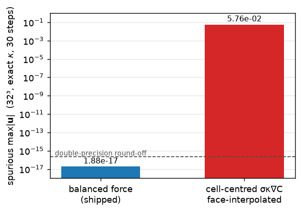
The balanced-force run sits at 1.88e-17 — below double-precision round-off on a field whose pressure is \(O(0.25)\), i.e. the velocity never left zero. The ablation sits at 5.76e-02, a factor 3.1e+15 larger. Both runs converged their pressure solve in a handful of iterations and carry a divergence at round-off, so neither is a solver artefact.
This is the whole content of “balanced force”, and it is worth stating plainly: the accuracy of the curvature has nothing to do with it. Equation 3 with a wrong-but-constant \(\kappa\) would still give machine zero. The failure mode of the ablation is structural, not quantitative.
2. With the computed curvature, Ca converges at second order
Now let the solver estimate its own curvature. peclet’s cascade (Popinet 2009) is a height function on 7-cell column sums of \(C\), falling back to a PLIC-volumetric paraboloid fit where the columns do not close — never a derivative of the reconstructed normal, which does not converge. Whatever error that estimator makes now enters Equation 3 as a \(\kappa_f\) that varies from face to face, so the force is no longer a discrete gradient, and the residue is the curvature error. In cell units \(\mathrm{Ca}\approx\delta\kappa\cdot h\).
We sweep the droplet diameter over \(D/\Delta = 8, 16, 24, 32\) (boxes \(16^3\) to \(64^3\), always \(D = n/2\) so the periodic images stay equally far away) and run 60 steps at each.
rungs = [(16, 4.0), (32, 8.0), (48, 12.0), (64, 16.0)]
sweep = [droplet(n, R) for n, R in rungs]
D = np.array([2 * R for _, R in rungs])
Ca = np.array([MU * r["umax"] / SIGMA for r in sweep])
order = -np.polyfit(np.log(D), np.log(Ca), 1)[0]

print(f"{'D/dx':>6} {'Ca':>11} {'ratio':>7} {'dkappa rms':>12} {'dkappa max':>11} "
      f"{'orphans':>9} {'pressure':>10} {'max|div|':>10}")
for i, ((n, R), r, ca) in enumerate(zip(rungs, sweep, Ca)):
    live = (r["branch"] > 0.5) & (r["branch"] < 5.5)
    dk = np.abs(r["kappa"][live] - 2.0 / R)
    ratio = f"{Ca[i-1]/ca:.2f}" if i else ""
    print(f"{2*R:6.0f} {ca:11.3e} {ratio:>7} "
          f"{dk.std():12.2e} {dk.max():11.2e} {str(r['csf']['orphan_faces']):>9} "
          f"{r['iters']:>7}/{r['cap']} {r['div']:10.1e}")
print(f"\nfitted order of Ca in D/dx: {order:.2f}")
D/dx Ca ratio dkappa rms dkappa max orphans pressure max|div|
8 2.543e-04 4.57e-03 3.57e-02 (0, 0, 0) 12/500 1.8e-15
16 5.898e-05 4.31 8.65e-04 5.54e-03 (0, 0, 0) 13/500 2.5e-16
24 2.649e-05 2.23 2.68e-04 1.70e-03 (1, 1, 1) 13/500 2.0e-16
32 1.388e-05 1.91 1.22e-04 8.06e-04 (0, 0, 0) 13/500 1.6e-16
fitted order of Ca in D/dx: 2.09from matplotlib.ticker import NullFormatter
Ca_exact = MU * exact[0]["umax"] / SIGMA
fig, (ax, axz) = plt.subplots(2, 1, figsize=(5.0, 4.4), sharex=True,
gridspec_kw=dict(height_ratios=[4, 1], hspace=0.12))
ax.loglog(D, Ca, "o-", color=BLUE, ms=7, lw=1.6, label="computed curvature")
fit = Ca[0] * (D / D[0]) ** (-order)
ax.loglog(D, fit, "--", color="0.35", lw=1.2, label=f"fitted order {order:.2f}")
ax.set_ylim(0.6 * Ca.min(), 2.0 * Ca.max())
ax.set_ylabel(r"$\mathrm{Ca} = \mu\,\max|u|/\sigma$")
ax.set_title("Parasitic currents vs droplet resolution")
ax.legend(fontsize=8, loc="upper right")
axz.set_xscale("log"); axz.set_yscale("log")
axz.plot([D[0] * 0.85, D[-1] * 1.18], [Ca_exact, Ca_exact], color=GREEN, lw=2.0)
axz.set_ylim(0.15 * Ca_exact, 7 * Ca_exact)
axz.set_yticks([Ca_exact]); axz.set_yticklabels([f"{Ca_exact:.0e}"])
axz.set_xticks(D); axz.set_xticklabels([f"{d:.0f}" for d in D])
axz.xaxis.set_minor_formatter(NullFormatter())
axz.set_xlabel(r"droplet resolution $D/\Delta$ [cells per diameter]")
axz.text(0.98, 0.62, "exact κ (machine zero)", transform=axz.transAxes,
ha="right", va="bottom", fontsize=8, color=GREEN)
# axis break marks
for a, y in ((ax, 0.0), (axz, 1.0)):
a.plot([0, 1], [y, y], transform=a.transAxes, color="w", lw=3, clip_on=False, zorder=5)
a.plot([-0.012, 0.012], [y - 0.02, y + 0.02], transform=a.transAxes,
color="0.3", lw=1, clip_on=False, zorder=6)
a.plot([0.988, 1.012], [y - 0.02, y + 0.02], transform=a.transAxes,
color="0.3", lw=1, clip_on=False, zorder=6)
plt.show()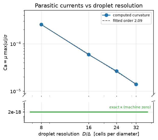
The headline: Ca falls from 2.54e-04 at 8 cells per diameter to 1.39e-05 at 32, a fitted order of 2.09 — second order, which is the convergence rate of the height-function curvature and therefore exactly what Equation 3 predicts once \(\kappa\) stops being exact.
NoteWhat this means for the pore scale
\(\mathrm{Ca}\approx\delta\kappa\,h\) in cell units, so a spurious-current budget is really a curvature requirement. A \(10^{-7}\) budget is not reachable by refining a static droplet forever either: with advection-realistic volume fractions — the ragged \(C\) a real transported interface carries, rather than the analytically exact fractions used here — the curvature error stops converging. The force is exact; the estimator is the ceiling.
3. The curvature branch census
compute_vof_curvature() fills two fields: kappa and kappa_branch, and the second is not optional reading. \(\kappa\) is 0 both where there is no interface (branch 0, correct) and where no estimate could be made (branch 6, which must never happen). Branches 1–2 are the height function, 4–5 the PLIC-volumetric paraboloid fallback.
NAMES = {0: "no interface", 1: "height function", 2: "HF, other direction",
         3: "mixed height-position (off)", 4: "PLIC paraboloid", 5: "PLIC, rank-deficient",
         6: "NO ESTIMATE (defect)"}
SHORT = {1: "HF", 2: "HF (other dir)", 4: "PLIC paraboloid", 5: "PLIC rank-def",
         6: "no estimate!"}
print(f"{'D/dx':>5} " + " ".join(f"{SHORT[b]:>16}" for b in (1, 2, 4, 5, 6))
      + f"{'fallback %':>12}")
for (n, R), r in zip(rungs, sweep):
    b = r["branch"]
    cnt = {k: int((np.abs(b - k) < 0.5).sum()) for k in (1, 2, 4, 5, 6)}
    live = sum(cnt.values())
    print(f"{2*R:5.0f} " + " ".join(f"{cnt[k]:>16d}" for k in (1, 2, 4, 5, 6))
          + f"{100*(cnt[4]+cnt[5])/live:11.1f}%")
D/dx HF HF (other dir) PLIC paraboloid PLIC rank-def no estimate! fallback %
8 91 0 223 0 0 71.0%
16 789 0 428 0 0 35.2%
24 1999 0 708 0 0 26.2%
32 3749 0 1079 0 0 22.3%fig, ax = plt.subplots(figsize=(5.2, 3.4))
keys = [1, 2, 4, 5]
cols = {1: BLUE, 2: "#7fb2dd", 4: RED, 5: "#f0928f"}
bottom = np.zeros(len(rungs))
for k in keys:
frac = np.array([100 * (np.abs(r["branch"] - k) < 0.5).sum()
/ ((r["branch"] > 0.5) & (r["branch"] < 5.5)).sum() for r in sweep])
ax.bar([f"{2*R:.0f}" for _, R in rungs], frac, bottom=bottom, color=cols[k],
label=NAMES[k], width=0.6)
bottom += frac
ax.set(xlabel=r"$D/\Delta$", ylabel="% of interfacial cells", ylim=(0, 100),
title="Curvature cascade: which branch served the cell")
ax.legend(fontsize=8, loc="upper center", bbox_to_anchor=(0.5, -0.16), ncol=2,
frameon=False)
ax.grid(axis="x", visible=False)
plt.show()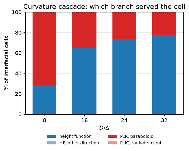
csf_diagnostics() also counts orphan faces — faces the colour jumps across but where neither cell carries a curvature estimate, so the force would have to be dropped. An orphan is a defect, and it is counted rather than hidden; the sweep above reports 0–1 per component at every rung.
4. The wisp guard: why a threshold on the predicate is not optional
Weymouth–Yue advection is exactly conservative, and the price is round-off colour residue: every cell its sweeps touch keeps a \(C\) of order \(10^{-30}\) (measured down to \(-3\times10^{-35}\)). Those cells satisfy the naive interfacial predicate \(0 < C < 1\), so the cascade dutifully builds a PLIC polygon of area \(\sim0\) for them and fits a paraboloid to it. A face between such a cell and a real interfacial cell then has \(\Delta C = O(1)\) and a face curvature \((\kappa_{\text{real}} + 10^{11})/2\).
The fix is a threshold on the predicate — a cell carries an interface only while \(\varepsilon < C < 1-\varepsilon\). set_surface_tension sets \(\varepsilon = 10^{-8}\); set_vof_interface_eps(0) restores the unguarded predicate, which is the ablation.
wisp = {}
for eps in (1e-8, 0.0):
    try:
        wisp[eps] = droplet(64, 16.0, steps=60, interface_eps=eps)
    except RuntimeError as e:                      # eps=0 can trip the WY CFL cap outright
        print(f"eps = {eps:g}: DIVERGED — {str(e)[:80]}")
W = {}
for eps, r in wisp.items():
    live = (r["branch"] > 0.5) & (r["branch"] < 5.5)
    W[eps] = dict(served=int(live.sum()), kmax=float(np.abs(r["kappa"][live]).max()),
                  u0=r["hist"][0], u1=r["hist"][-1])
    print(f"eps = {eps:<6g}  max|u| step 1 {r['hist'][0]:.3e} -> step 60 {r['hist'][-1]:.3e}"
          f"   cells served {W[eps]['served']:5d}   max|kappa| {W[eps]['kmax']:.3e}"
          f"   (physical 2/R = {2/16.0:.4f})")
eps = 1e-08 max|u| step 1 2.110e-03 -> step 60 1.388e-04 cells served 4828 max|kappa| 1.258e-01 (physical 2/R = 0.1250)
eps = 0 max|u| step 1 2.110e-03 -> step 60 1.853e-03 cells served 10018 max|kappa| 2.868e+11 (physical 2/R = 0.1250)fig, ax = plt.subplots(figsize=(5.0, 3.6))
lbl = {1e-8: r"$\varepsilon = 10^{-8}$ (default, guarded)", 0.0: r"$\varepsilon = 0$ (unguarded)"}
for eps, col in ((1e-8, BLUE), (0.0, RED)):
if eps in wisp:
ax.semilogy(np.arange(1, len(wisp[eps]["hist"]) + 1), wisp[eps]["hist"],
color=col, lw=1.7, label=lbl[eps])
ax.set(xlabel="step", ylabel=r"$\max|\mathbf{u}|$",
title="Spurious velocity with and without the wisp guard")
ax.legend(fontsize=9)
plt.show()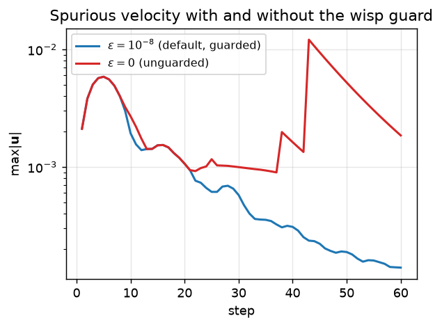
Guarded, max|u| decays from 2.11e-03 to 1.39e-04 over 60 steps and the largest curvature in the field is 0.1258, against the physical \(2/R = 0.125\). Unguarded, the same run serves 10018 cells instead of 4828 — more “interfacial” cells than the interface has — reports a maximum curvature of 2.87e+11, and the velocity does not decay (2.11e-03 at step 1 against 1.85e-03 at step 60). This is the trap the literature knows as “with surface tension some clipping is unavoidable” (Arrufat et al. 2021), arriving in the cheapest available form.
Collocated cross-check
peclet also ships a cell-centred/collocated grid (flow.SolverColocated), and since rung V8 it runs two-phase flow too. Its projection is approximate (ABC): the cell velocities are averaged onto a MAC face field, that field is projected exactly, and the correction is averaged back. That moves where the balanced-force identity lives, and it changes which number you are allowed to quote.
On this grid every interfacial force is applied as a face acceleration \(a_f = \Delta t\,(\sigma\kappa_f\,\Delta_f C/h - \Delta_f P)/\rho_f\), added after the cell-to-face average, and the cell takes the average of its two faces’ total increment — Basilisk’s centered.h construction (Popinet 2009). A cell-centred \(\sigma\kappa\nabla C/\rho_c\) would be \(O(1)\) wrong at an interface cell even when every face is exactly balanced, which is Equation 3’s lesson one level up. The switch is one argument: droplet(..., cls=flow.SolverColocated) — the driver above takes the solver class, and nothing else changes.
NoteRead the FACE field on this grid
A cell-field checkerboard is annihilated by the cell-to-face average \(\tfrac12(U_i + U_{i-1})\), so the approximate projection is structurally blind to it and cannot remove it. The spurious-current number on the collocated grid is therefore the one on get_uf/get_vf/get_wf; the cell number is printed beside it and carries that invisible mode as well.
CO = flow.SolverColocated
co_exact = droplet(32, 8.0, steps=30, exact_kappa=True, cls=CO)
print("exact curvature, uniform rho, 32^3, R = 8, 30 steps")
for lab, r in (("staggered", exact[0]), ("collocated", co_exact)):
    print(f"  {lab:>10}   cell max|u| {r['umax']:.4e}   face max|uf| {r['ufmax']:.4e}"
          f"   pressure {r['iters']}/{r['cap']}   max|div| {r['div']:.1e}")
peclet::flow SolverColocated: AUTO scheme fell back to gauge-exact (geometric VoF on the collocated grid is rung V8 and the ghost projection v1 does not support it). Select explicitly with set_collocated_scheme to silence this notice.exact curvature, uniform rho, 32^3, R = 8, 30 steps
staggered cell max|u| 1.8781e-17 face max|uf| 1.8781e-17 pressure 13/500 max|div| 2.7e-16
collocated cell max|u| 2.7974e-17 face max|uf| 3.0208e-17 pressure 13/500 max|div| 3.0e-16The exactness identity survives the move: with an exact \(\kappa\) the collocated face field sits at 3.02e-17 and its cell field at 2.80e-17, against the staggered 1.88e-17 — all three below double-precision round-off on a field whose pressure is \(O(0.25)\). Nothing is being hidden by an averaging operator: the face balance is exact, and the cell sees the average of an exact zero.
co_sweep = {2 * R: droplet(n, R, cls=CO) for n, R in rungs[:2]}
print(f"{'D/dx':>6} {'staggered Ca':>14} {'collocated Ca (cell)':>22} "
      f"{'collocated Ca (face)':>22} {'collocated/staggered':>21}")
for (n, R), a in zip(rungs[:2], sweep[:2]):
    b = co_sweep[2 * R]
    s_, c_, f_ = MU * a["umax"] / SIGMA, MU * b["umax"] / SIGMA, MU * b["ufmax"] / SIGMA
    print(f"{2*R:6.0f} {s_:14.3e} {c_:22.3e} {f_:22.3e} {c_/s_:20.2f}x")
CA8 = MU * co_sweep[8.0]["umax"] / SIGMA / Ca[0]
CA16 = MU * co_sweep[16.0]["umax"] / SIGMA / Ca[1]
peclet::flow SolverColocated: AUTO scheme fell back to gauge-exact (geometric VoF on the collocated grid is rung V8 and the ghost projection v1 does not support it). Select explicitly with set_collocated_scheme to silence this notice.
peclet::flow SolverColocated: AUTO scheme fell back to gauge-exact (geometric VoF on the collocated grid is rung V8 and the ghost projection v1 does not support it). Select explicitly with set_collocated_scheme to silence this notice. D/dx staggered Ca collocated Ca (cell) collocated Ca (face) collocated/staggered
8 2.543e-04 2.018e-04 1.942e-04 0.79x
16 5.898e-05 4.834e-05 4.706e-05 0.82xWith the estimator back in the loop the collocated grid is not worse — it is slightly better, 0.82× the staggered \(\mathrm{Ca}\) at \(D/\Delta = 16\) and 0.79× at 8. That is the ceiling of §2 showing itself again: on both grids these numbers are the curvature error, and both grids call the same cascade.
Where the collocated rung stops
What does not carry over is the density ratio. Repeat the exact-\(\kappa\) droplet with the gas held at \(\rho = 1\) and the drop at $= $ ratio, so that \(\rho_{\min}\) is fixed and only the capillary time step grows:
def face_num(**kw):
try:
return f"{droplet(32, 8.0, steps=30, exact_kappa=True, **kw)['ufmax']:.4e}"
except RuntimeError:
return "UNSTABLE"
rows = [] # collected first, printed once: the solver writes a
for ratio, mu in ((1.0, MU), (10.0, MU), # scheme notice to stderr on every collocated build
(100.0, MU), (1000.0, MU), (1000.0, 0.01)):
dt = 0.5 * np.sqrt((1.0 + ratio) / (4 * np.pi)) # the Brackbill limit at rho_gas = 1
rows.append(f"{ratio:7.0f} {mu:6g} {face_num(ratio=ratio, mu=mu):>16} "
f"{face_num(ratio=ratio, mu=mu, cls=CO):>17} {mu*dt:23.2f}")
print(f"{'ratio':>7} {'mu':>6} {'staggered face':>16} {'collocated face':>17} "
f"{'mu dt / (rho_gas h^2)':>23}")
print("\n".join(rows))peclet::flow SolverColocated: AUTO scheme fell back to gauge-exact (geometric VoF on the collocated grid is rung V8 and the ghost projection v1 does not support it). Select explicitly with set_collocated_scheme to silence this notice.
peclet::flow SolverColocated: AUTO scheme fell back to gauge-exact (geometric VoF on the collocated grid is rung V8 and the ghost projection v1 does not support it). Select explicitly with set_collocated_scheme to silence this notice.
peclet::flow SolverColocated: AUTO scheme fell back to gauge-exact (geometric VoF on the collocated grid is rung V8 and the ghost projection v1 does not support it). Select explicitly with set_collocated_scheme to silence this notice.
peclet::flow SolverColocated: AUTO scheme fell back to gauge-exact (geometric VoF on the collocated grid is rung V8 and the ghost projection v1 does not support it). Select explicitly with set_collocated_scheme to silence this notice.
peclet::flow SolverColocated: AUTO scheme fell back to gauge-exact (geometric VoF on the collocated grid is rung V8 and the ghost projection v1 does not support it). Select explicitly with set_collocated_scheme to silence this notice. ratio mu staggered face collocated face mu dt / (rho_gas h^2)
1 0.1 1.8781e-17 3.0208e-17 0.02
10 0.1 2.0374e-05 1.0015e-11 0.05
100 0.1 1.8377e-05 1.7690e-06 0.14
1000 0.1 1.0485e-05 UNSTABLE 0.45
1000 0.01 4.6552e-06 6.8386e-11 0.04Ratio 1000 at \(\mu = 0.1\) fails on the collocated grid: instead of sitting at rest the run trips the Weymouth–Yue Courant cap after about fifteen steps. The mechanism is worth stating, because it is not the density ratio itself. On the staggered grid the force enters the right-hand side of the momentum solve, so \(A^{-1}\) with \(A = \rho_f/\Delta t - \mu\nabla^2\) damps its high-wavenumber content — the damping that makes the staggered balance slightly inexact at variable \(\rho\) (the \(\mu\,\Delta t^2\) residue in “Adapt this yourself”) is also what stabilises it. Applying the force at the face, outside \(A\), buys the exact balance — the collocated column is four to six orders better at ratios 10 and 100 — and pays for it by advancing the face and the cell with different operators. The mismatch is governed by \(\mu\,\Delta t/(\rho_{\min}h^2)\), printed in the last column: at ratio 1000 the capillary step has grown by \(\sqrt{1001}\) while \(\rho_{\min}\) has not, and the run is past the edge. Drop \(\mu\) to \(0.01\) at the same ratio and it is back at \(10^{-10}\).
Practical rating: use the collocated grid for two-phase work at density ratio \(\lesssim 100\), or higher with \(\mu\,\Delta t/(\rho_{\min}h^2)\lesssim 0.05\). The staggered grid is the reference for everything else, and it is what the rest of this page measures.
Adapt this yourself
- Change the density ratio.
set_property_model("rho", "linear", "C", [rho_g, rho_l-rho_g])makes this a real two-phase droplet. The equilibrium is then approached rather than hit: the semi-implicit momentum operator \(A = \rho_f/\Delta t - \mu\nabla^2\) commutes with the discrete gradient only at constant \(\rho_f\), so a residue of order \(\mu\,\Delta t^2\) appears at the first step and then decays. - Change the viscosity. With an exact curvature the machine-zero result is independent of \(\mu\) over four decades — a good check that your build is healthy.
- Freeze the curvature instead of making it exact.
set_vof_kappa_frozen(True)keeps whatever is in thekappafield, which separates “the estimator is wrong” from “the estimator is fed back through the transport”. - Push the resolution. \(D/\Delta = 48\) needs a \(96^3\) box; on a CUDA build that is still seconds per run, and it extends the log-log fit by another point.
- Go multi-rank. The identical script runs under
mpirun -np N python …; the curvature cascade reaches exactly \(\pm3\) cells, which is the colour field’s own ghost depth, so no reduction appears anywhere in it and the result is bitwise decomposition-independent at np = 1.
Reproduce this
The compiled solver runs this, so its outputs are frozen into the site. To regenerate:
pip install peclet            # the solver, from PyPI
quarto render examples/parasitic-currents/index.qmd --execute
# ...or against a local source build of the suite (GPU):
PECLET_LOCAL_BUILD=/path/to/suite/flow/build_cuda OMP_NUM_THREADS=8 OMP_PROC_BIND=false \
  quarto render examples/parasitic-currents/index.qmd --execute
The same battery is available inside the solver repo as tests/study/vof_surface_tension.py static, and its algebraic siblings (the exactness gate, Young–Laplace to \(2\times10^{-16}\), the capillary time step, inertness when surface tension is off) run in the vof_surface_tension ctest.
References
Arrufat, T., M. Crialesi-Esposito, D. Fuster, et al. 2021. “A Mass-Momentum Consistent, Volume-of-Fluid Method for Incompressible Flow on Staggered Grids.” Computers & Fluids 215: 104785. https://doi.org/10.1016/j.compfluid.2020.104785.
Brackbill, J. U., D. B. Kothe, and C. Zemach. 1992. “A Continuum Method for Modeling Surface Tension.” Journal of Computational Physics 100 (2): 335–54. https://doi.org/10.1016/0021-9991(92)90240-Y.
Francois, Marianne M., Sharen J. Cummins, Edward D. Dendy, Douglas B. Kothe, James M. Sicilian, and Matthew W. Williams. 2006. “A Balanced-Force Algorithm for Continuous and Sharp Interfacial Surface Tension Models Within a Volume Tracking Framework.” Journal of Computational Physics 213 (1): 141–73. https://doi.org/10.1016/j.jcp.2005.08.004.
Popinet, Stéphane. 2009. “An Accurate Adaptive Solver for Surface-Tension-Driven Interfacial Flows.” Journal of Computational Physics 228 (16): 5838–66. https://doi.org/10.1016/j.jcp.2009.04.042.