import importlib.util, os, subprocess, sys
_local = os.environ.get("PECLET_LOCAL_BUILD")
if _local:
    sys.path.insert(0, _local)
elif importlib.util.find_spec("peclet") is None:
subprocess.run([sys.executable, "-m", "pip", "install", "-q", "peclet"], check=True)Pipe flow: second-order convergence on a curved wall
Hagen–Poiseuille through a cylindrical SDF pipe — where the curved boundary finally costs you O(h²).
flow
IBM
cut-cell
SDF
convergence
 Runs on a free Colab CPU runtime — the first cell installs
 peclet from PyPI.
What you’ll learn
The companion to the plane-channel example, and a sharper test of the cut-cell IBM. Pipe (Hagen–Poiseuille) flow has the same parabolic velocity profile as the plane channel — so you might expect the same machine-exact result. It isn’t: the pipe wall is curved, and a curved boundary cannot be represented exactly on a Cartesian grid. The consequence is a genuine second-order (\(\mathcal{O}(h^2)\)) error — the convergence study the plane channel could never show, because there the answer was already exact.
The problem
A body force \(F\) drives flow along a cylindrical pipe of radius \(R\). The steady axial velocity is the paraboloid
\[ u(r) = \frac{F}{4\mu}\,(R^2 - r^2), \qquad U_{\max} = \frac{F R^2}{4\mu}, \tag{1}\]
with \(r\) the distance from the axis. Like the plane channel this is quadratic — but now quadratic in two transverse coordinates, and the no-slip circle \(r=R\) slices diagonally through Cartesian cells. The cut-cell IBM approximates that circle to \(\mathcal{O}(h^2)\), and that geometric error sets the accuracy.
import numpy as np
import matplotlib.pyplot as plt
from peclet import flow

plt.rcParams.update({"figure.dpi": 130, "font.size": 10, "axes.grid": True,
                     "grid.alpha": 0.3, "axes.axisbelow": True,
                     "figure.facecolor": "white", "savefig.bbox": "tight"})
BLUE, RED = "#1f77b4", "#d62728"
Geometry: a cylinder as an SDF
The pipe axis runs along \(x\) (periodic). In each \(y\)–\(z\) cross-section the fluid is the disk \(r<R\); the SDF is R - r, positive inside the pipe and negative in the surrounding solid.
def pipe_sdf(nx, N, R):
    """sdf[x,y,z] = R - r, >0 inside the pipe (fluid), <0 in the solid; axis along x."""
    g = np.arange(N) + 0.5                       # cell centres
    c = N / 2.0
    Y, Z = np.meshgrid(g, g, indexing="ij")
    r = np.sqrt((Y - c) ** 2 + (Z - c) ** 2)
    sdf2 = R - r
    return np.asfortranarray(np.repeat(sdf2[None, :, :], nx, axis=0)), r, c
Solve, and compare to the paraboloid
def solve_pipe(N, Rfrac=0.40, F=1e-3, mu=0.1, nx=6, dt=50.0, max_steps=400):
    R = Rfrac * N
    sdf, r, c = pipe_sdf(nx, N, R)
    s = flow.Solver(nx, N, N)
    s.set_rho(1.0); s.set_mu(mu); s.set_dt(dt)
    s.set_body_force(F, 0.0, 0.0)
    s.set_velocity_solver_params(120)
    s.set_pressure_solver_params(1)              # axially uniform -> projection is a no-op
    s.set_solid(sdf, cutcell_pressure=False)
    prev = 0.0
    for it in range(max_steps):
        s.step()
        m = float(s.get_u().max())
        if it > 10 and abs(m - prev) < 1e-10 * (abs(m) + 1e-12):
            break
        prev = m
    u = s.get_u()[nx // 2]                        # (N,N) cross-section
    ana = np.where(r < R, F / (4 * mu) * (R ** 2 - r ** 2), 0.0)
    fluid = r < R
    Umax_ana = F * R ** 2 / (4 * mu)
    rel_err = float(np.max(np.abs(u[fluid] - ana[fluid])) / Umax_ana)
    return dict(N=N, R=R, r=r, c=c, u=u, ana=ana, fluid=fluid,
                rel_err=rel_err, Umax_ana=Umax_ana, iters=it)

res = [solve_pipe(N) for N in (16, 24, 32, 48)]
for d in res:
    print(f"N={d['N']:3d}  R={d['R']:5.1f}  rel error = {d['rel_err']:.3e}   "
          f"U_max: sim={d['u'][d['fluid']].max():.5f}  analytic={d['Umax_ana']:.5f}")
N= 16 R= 6.4 rel error = 1.367e-03 U_max: sim=0.10107 analytic=0.10240
N= 24 R= 9.6 rel error = 1.112e-03 U_max: sim=0.22905 analytic=0.23040
N= 32 R= 12.8 rel error = 4.017e-04 U_max: sim=0.40827 analytic=0.40960
N= 48 R= 19.2 rel error = 2.019e-04 U_max: sim=0.92026 analytic=0.92160The cross-section and the radial collapse
The velocity is an axisymmetric paraboloid. Plotting every fluid node’s velocity against its radius collapses the whole 2-D field onto the analytic curve — with a faint spread near the wall, the signature of the cut-cell boundary approximation.
d = res[-1]
fig, (axl, axr) = plt.subplots(1, 2, figsize=(9.0, 3.8))

um = np.where(d["fluid"], d["u"], np.nan)
im = axl.imshow(um.T, origin="lower", cmap="viridis")
axl.set(title=f"axial velocity, N={d['N']}", xlabel="y", ylabel="z")
axl.grid(False)
fig.colorbar(im, ax=axl, fraction=0.046, pad=0.04, label="u")

rr = d["r"][d["fluid"]]; uu = d["u"][d["fluid"]]
rc = np.linspace(0, d["R"], 200)
axr.scatter(rr, uu, s=6, color=BLUE, alpha=0.35, label="fluid nodes")
axr.plot(rc, d["Umax_ana"] * (1 - (rc / d["R"]) ** 2), "-", color="0.15", lw=1.6,
         label="analytic paraboloid")
axr.set(title="radial collapse", xlabel="r (distance from axis)", ylabel="u")
axr.legend(fontsize=8)
fig.tight_layout()
plt.show()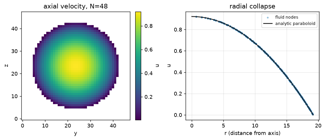
Second-order convergence
Refining the grid (larger \(N\) at fixed \(R/N\)) shrinks the error at the scheme’s true rate. The fitted slope is close to \(-2\): the curved-wall cut-cell IBM is second-order accurate.
Ns = np.array([d["N"] for d in res])
errs = np.array([d["rel_err"] for d in res])
order = np.polyfit(np.log(Ns), np.log(errs), 1)[0]

fig, ax = plt.subplots(figsize=(5.0, 3.8))
ax.loglog(Ns, errs, "o-", color=RED, label="measured error")
ax.loglog(Ns, errs[0] * (Ns / Ns[0]) ** -2.0, "k--", label=r"$\mathcal{O}(h^2)$")
ax.set(xlabel="N (pipe diameter in cells)", ylabel="relative velocity error",
       title=f"Cut-cell IBM convergence — fitted order {order:.2f}")
ax.legend()
plt.show()

print(f"fitted convergence order = {order:.2f}   (curved wall -> second order)")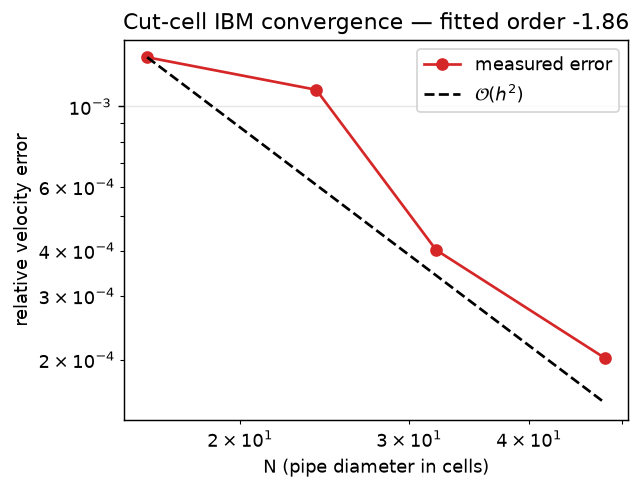
fitted convergence order = -1.86 (curved wall -> second order)The takeaway
Same parabolic physics, two very different verdicts:
| wall | representation | result | |
|---|---|---|---|
| Plane channel | flat | exact | machine-exact at every N |
| Pipe (here) | curved | \(\mathcal{O}(h^2)\) | second-order convergent |
The lesson: the cut-cell IBM is second-order, and for geometry it can represent exactly (flat, axis-aligned) it is exactly exact. Curvature is where the order becomes visible — which is exactly why the genuine convergence benchmarks in this gallery (the Zick–Homsy sphere arrays) use curved solids.
Adapt this yourself
- Elliptical or eccentric pipe. Change
pipe_sdfto an ellipse or offset the centre — the analytic profile changes but the method doesn’t. - Resolve the wall better. Increase
Rfrac(more cells across the pipe) to push the error down along the \(\mathcal{O}(h^2)\) line. - Add inertia. Raise the body force / lower
muand switch on advection (set_advection(True)) to develop the entrance region in a finite-length pipe.
Reproduce this
pip install peclet
quarto render examples/pipe-poiseuille/index.qmd --execute
# ...or against a local source build:
PECLET_LOCAL_BUILD=/path/to/suite/flow/build_mpi OMP_NUM_THREADS=4 \
  quarto render examples/pipe-poiseuille/index.qmd --execute