import importlib.util, os, subprocess, sys
_local = os.environ.get("PECLET_LOCAL_BUILD")
if _local:
    for p in _local.split(":"):
        sys.path.insert(0, p)
elif importlib.util.find_spec("peclet") is None:
subprocess.run([sys.executable, "-m", "pip", "install", "-q", "peclet"], check=True)Staggered vs collocated: grid convergence of Stokes drag
Two velocity placements × two cut-cell projections on the Zick–Homsy sphere array. The aperture cut-cell scheme converges at second order on the staggered grid but first order on the collocated grid; the directional ghost-cell projection is second order on both — closing the collocated gap.
flow
accuracy
staggered
collocated
ghost-cell
Stokes
verification
 Runs on a free Colab CPU runtime — the first cell installs
 peclet from PyPI.
What this measures
peclet.flow ships two velocity placements behind one identical Python API:
flow.Solver— the staggered MAC grid (velocities on cell faces, pressure at centres). The default, and the flow solver: exact discrete projection.flow.SolverColocated— a collocated grid (velocities and pressure both at cell centres) closed with an ABC approximate projection.
and, on each placement, two cut-cell treatments of the immersed boundary in the pressure projection:
- the aperture cut-cell scheme (default): the incompressibility constraint uses the fluid area fraction of every cut face (finite-volume flux throttling), solved by a symmetric multigrid-preconditioned CG;
- the directional ghost-cell scheme (
set_ghost_projection(True, 1, 2)): a point-based finite-difference divergence whose solid faces are closed by the same wall-anchored quadratics the momentum IBM uses, solved by multigrid-preconditioned BiCGStab. One consistent finite-difference family for no-slip, pressure force and constraint.
That is a 2×2 matrix of solvers over the same equations and the same geometry. This page puts all four under a microscope on a problem with an external ground truth — creeping flow through a periodic simple-cubic sphere array, whose Stokes drag Zick & Homsy (1982) computed semi-analytically. We refine the mesh and ask, for each combination:
- Does it converge, and at what order?
- To what value does it converge — the benchmark, or something offset from it?
- What does it cost (pressure iterations, wall-clock) to get there?
The punchline: the aperture cut-cell scheme is second order on the staggered grid but first order on the collocated grid (a half-cell wall-representation mismatch plus a pressure-gradient defect at cut cells — see What it means), while the ghost-cell projection is second order on both — it closes the collocated gap and lands on the benchmark with fewer pressure iterations. Getting this right needed resolutions up to \(N=128\) on a GPU; the coarse grids alone are genuinely ambiguous.
The drag factor
A body force \(F\) drives Stokes flow (no inertia) through a periodic cell of side \(L\) containing one sphere of radius \(R\) at solid fraction \(\phi=\tfrac{4}{3}\pi R^3/L^3\). The mean (superficial) velocity \(\langle u\rangle\) fixes the dimensionless drag factor — the per-sphere drag normalised by the isolated Stokes drag \(6\pi\mu R\langle u\rangle\):
\[ K=\frac{F\,L^{3}}{6\pi\mu R\,\langle u\rangle}, \tag{1}\]
which Zick & Homsy tabulate versus \(\phi\). At \(\phi=0.125\) (radius a quarter of the cell) their value is \(K_\text{ZH}=4.292\) — the target all four solvers must hit.
import time
import numpy as np
import matplotlib.pyplot as plt
from peclet import flow

plt.rcParams.update({"figure.dpi": 130, "font.size": 10, "axes.grid": True,
                     "grid.alpha": 0.3, "axes.axisbelow": True,
                     "figure.facecolor": "white", "savefig.bbox": "tight"})
BLUE, RED = "#1f77b4", "#d62728"

PHI0  = 0.125                    # solid fraction (sphere radius = L/4)
K_ZH  = 4.292                    # Zick & Homsy (1982), simple cubic, at PHI0
CENTRE = [(0.5, 0.5, 0.5)]       # one sphere per period, cell-centred

# the ghost projection ships with peclet-flow > 0.1 wheels; degrade gracefully on older ones
HAS_GHOST = hasattr(flow.Solver(4, 4, 4), "set_ghost_projection")
print("ghost projection available:", HAS_GHOST)
ghost projection available: TrueThe characterization harness
The same driver runs all four combinations — the only things that change between sweeps are the solver class and the ghost switch. It builds the sphere as a signed distance field, drives Stokes flow to a steady state, and reports the drag factor.
Because the collocated grid’s approximate projection leaves the mean velocity with a small residual jitter (the staggered grid’s exact projection does not), we detect a moderate steady state and then report \(\langle u\rangle\) averaged over a tail of steps — a fair, reproducible number for every variant rather than a single jittering sample.
def sphere_sdf(N, phi, centres):
    """SDF of a periodic sphere lattice on an N³ grid (negative inside a sphere)."""
    n = len(centres)
    R = (3 * phi / (4 * np.pi * n)) ** (1 / 3) * N
    g = np.arange(N) + 0.5
    X, Y, Z = np.meshgrid(g, g, g, indexing="ij")
    best = np.full((N, N, N), 1e30)
    for cx, cy, cz in centres:
        dx = X - cx * N; dx -= N * np.round(dx / N)
        dy = Y - cy * N; dy -= N * np.round(dy / N)
        dz = Z - cz * N; dz -= N * np.round(dz / N)
        best = np.minimum(best, np.sqrt(dx * dx + dy * dy + dz * dz) - R)
    return best, R

def drag(SolverCls, N, ghost=False, phi=PHI0, centres=CENTRE, mu=0.1, F=1e-3,
         dt=80.0, warm_tol=1e-6, tail=40, max_steps=1000):
    sdf, R = sphere_sdf(N, phi, centres)
    s = SolverCls(N, N, N)
    s.set_rho(1.0); s.set_mu(mu); s.set_dt(dt)
    s.set_body_force(F, 0, 0); s.set_advection(False)     # Stokes: inertia off
    s.set_velocity_solver_params(150)
    s.set_pressure_multigrid(True, levels=max(2, int(np.log2(N)) - 1))
    s.set_pressure_pcg(True, 200, 1e-8)
    if ghost:
        s.set_ghost_projection(True, 1, 2)   # (matrix, rhs) closure orders: the mixed default
    s.set_solid(sdf, cutcell_pressure=True, pressure_coarse="rediscretized")

    prev, warm, um, pit, t0 = 0.0, None, [], [], time.time()
    for it in range(max_steps):
        s.step()
        um.append(float(s.get_u().mean()))            # rolling history of <u>
        pit.append(int(s.last_pressure_iterations()))
        if warm is None:                              # still relaxing to steady state
            if it % 10 == 9:
                if it > 10 and abs(um[-1] - prev) < warm_tol * (abs(um[-1]) + 1e-30):
                    warm = it                         # reached moderate steady state
                prev = um[-1]
        elif it - warm >= tail:                       # collected a full post-warm tail
            break

    umean = float(np.mean(um[-tail:]))                # tail-average damps the jitter
    K = F * N ** 3 / len(centres) / (6 * np.pi * mu * R * umean)
    return dict(N=N, K=K, k=mu * umean / F, steps=it + 1, warm=warm,
                pit=float(np.mean(pit[-tail:])), secs=time.time() - t0)
Sweep the 2×2 matrix live
Ns = [16, 24, 32, 40]
grids = {"stag cutcell": (flow.Solver, False), "col cutcell": (flow.SolverColocated, False)}
if HAS_GHOST:
    grids |= {"stag ghost": (flow.Solver, True), "col ghost": (flow.SolverColocated, True)}
data = {name: [drag(cls, N, ghost=g) for N in Ns] for name, (cls, g) in grids.items()}

for name, rows in data.items():
    print(f"{name:>13s}: " + "  ".join(
        f"N={r['N']}→K={r['K']:.4f}({100*(r['K']-K_ZH)/K_ZH:+.2f}%)" for r in rows))
stag cutcell: N=16→K=4.2174(-1.74%) N=24→K=4.2609(-0.72%) N=32→K=4.2785(-0.31%) N=40→K=4.2843(-0.18%)
col cutcell: N=16→K=4.3254(+0.78%) N=24→K=4.3375(+1.06%) N=32→K=4.3343(+0.99%) N=40→K=4.3232(+0.73%)
stag ghost: N=16→K=4.1820(-2.56%) N=24→K=4.2411(-1.19%) N=32→K=4.2658(-0.61%) N=40→K=4.2752(-0.39%)
col ghost: N=16→K=4.2665(-0.59%) N=24→K=4.2791(-0.30%) N=32→K=4.2845(-0.18%) N=40→K=4.2867(-0.12%)Push to finer grids (the part that needs a GPU)
The live sweep above stops at \(N=40\) so it runs on a Colab CPU. But the coarse grids are genuinely ambiguous: at \(N\le40\) the collocated cut-cell error looks like it might be levelling off at ~1%, and you can’t tell “slowly converging” from “stuck at a floor”. The resolutions below — up to \(N=128\), run to a tight steady state with the same harness (warm_tol=1e-7, up to 4000 steps) — were computed on an RTX 5080 GPU and are quoted here as data (the Reproduce this section gives the exact scripts). They are the numbers that settle the question.
# Signed error (K - K_ZH)/K_ZH in %, RTX 5080, tight steady protocol (warm_tol 1e-7, tail 40).
# Columns: (stag cutcell, stag ghost, col cutcell, col ghost) per resolution.
HIRES = {
    32:  (-0.314, -0.610, +1.004, -0.175),
    48:  (-0.082, -0.257, +0.685, -0.084),
    64:  (-0.018, -0.144, +0.598, -0.056),
    96:  (+0.009, -0.066, +0.397, -0.029),
    128: (+0.013, -0.039, +0.299, -0.018),
}
NAMES = ["stag cutcell", "stag ghost", "col cutcell", "col ghost"]
allN = np.array(sorted(HIRES), float)
E = {n: np.array([HIRES[int(N)][i] for N in allN]) for i, n in enumerate(NAMES)}
Observed order of accuracy
With the full range in hand, read the local order between successive resolutions, \(p=\log(|e_{i-1}|/|e_i|)\,/\,\log(N_i/N_{i-1})\). Two caveats keep the reading honest: Richardson orders are meaningless where a signed error crosses zero (the staggered cut-cell error does, near \(N\approx96\)), and drag errors below \(\sim0.05\%\) are under the precision of the Zick–Homsy table itself — both ghost columns reach that floor.
hdr = f"{'N pair':>10} |" + "".join(f" {n:>13} |" for n in NAMES)
print(hdr)
for i in range(1, len(allN)):
    row = f"{int(allN[i-1]):>4}->{int(allN[i]):<4} |"
    for n in NAMES:
        p = np.log(abs(E[n][i-1]) / abs(E[n][i])) / np.log(allN[i] / allN[i-1])
        row += f" {p:>+13.2f} |"
    print(row)
N pair | stag cutcell | stag ghost | col cutcell | col ghost |
32->48 | +3.31 | +2.13 | +0.94 | +1.81 |
48->64 | +5.27 | +2.01 | +0.47 | +1.41 |
64->96 | +1.71 | +1.92 | +1.01 | +1.62 |
96->128 | -1.28 | +1.83 | +0.99 | +1.66 |The result
fig, (a0, a1) = plt.subplots(1, 2, figsize=(11, 4.1))
style = {"stag cutcell": (BLUE, "o", "-"), "stag ghost": (BLUE, "^", "--"),
         "col cutcell": (RED, "s", "-"), "col ghost": (RED, "v", "--")}

a0.axhline(0, color="0.4", ls="--", lw=1)
for n in NAMES:
    c, m, ls = style[n]
    a0.plot(allN, E[n], marker=m, ls=ls, color=c, label=n)
a0.set(xlabel="N (cells per period)", ylabel="(K − K$_{ZH}$) / K$_{ZH}$  [%]",
       title="signed error → 0 for all four")
a0.legend(fontsize=8)

for n in NAMES:
    c, m, ls = style[n]
    a1.loglog(allN, np.abs(E[n]), marker=m, ls=ls, color=c, label=n)
a1.loglog(allN, abs(E["col cutcell"][0]) * (allN / allN[0]) ** -1.0, ":",
          color="0.5", lw=1.2, label="O(h¹)")
a1.loglog(allN, abs(E["col ghost"][0]) * (allN / allN[0]) ** -2.0, "k--",
          lw=1, label="O(h²)")
a1.set(xlabel="N", ylabel="|K − K$_{ZH}$| / K$_{ZH}$  [%]",
       title="col cutcell ∥ O(h); the other three ∥ O(h²)")
a1.legend(fontsize=7)
fig.tight_layout()
plt.show()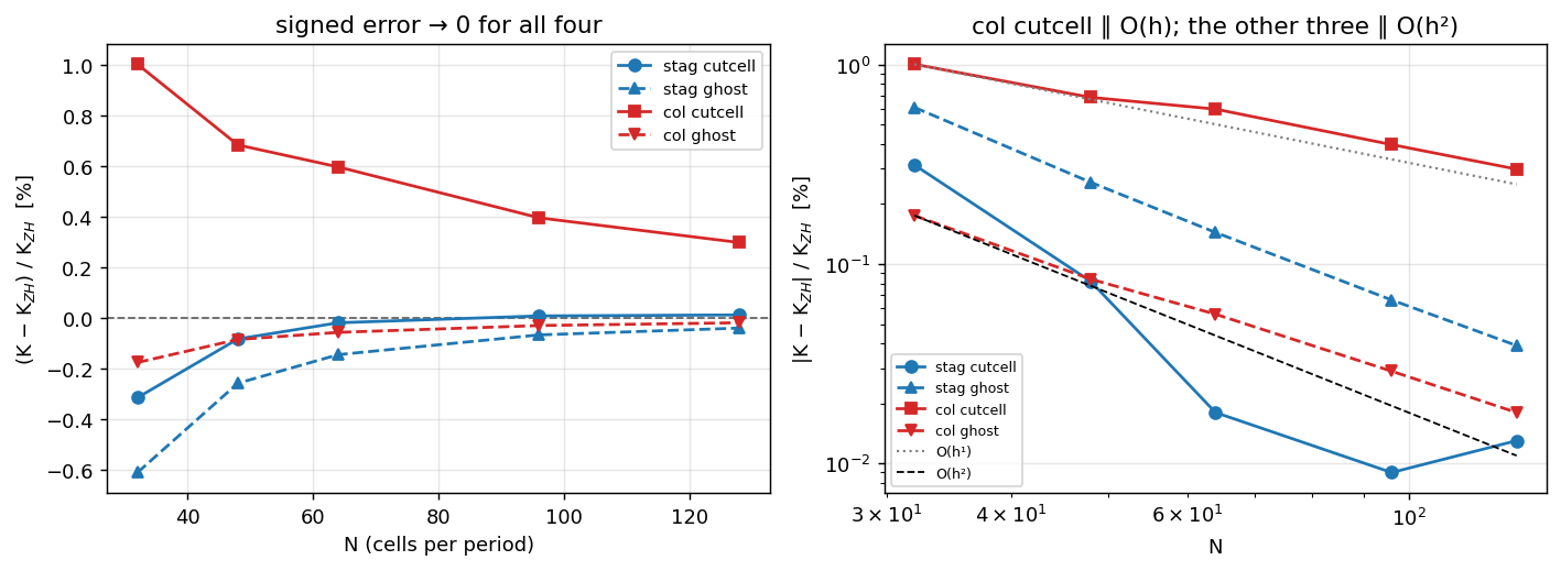
Performance: what each projection costs
Accuracy is only half the choice; the two projections also solve different linear systems. The aperture scheme’s operator is symmetric positive-semidefinite — multigrid-preconditioned CG, one matvec + one V-cycle per iteration. The ghost scheme’s operator is mildly nonsymmetric (the directional closures) — multigrid- preconditioned BiCGStab, two matvecs + two V-cycles per iteration. Iteration counts per time step, measured over the steady tail of the GPU runs above:
# mean pressure-solver iterations per step over the steady tail (RTX 5080 runs above)
ITERS = {  # N: (stag cutcell CG, stag ghost BiCGStab, col cutcell CG, col ghost BiCGStab)
    32:  (9, 6, 10, 6),
    64:  (9, 7, 10, 7),
    128: (9, 7, 10, 7),
}
print(f"{'N':>5} |" + "".join(f" {n:>13} |" for n in NAMES))
for N, row in ITERS.items():
    print(f"{N:>5} |" + "".join(f" {v:>13} |" for v in row))
N | stag cutcell | stag ghost | col cutcell | col ghost |
32 | 9 | 6 | 10 | 6 |
64 | 9 | 7 | 10 | 7 |
128 | 9 | 7 | 10 | 7 |Reading it with the 2 V-cycles/iteration factor in mind: the ghost BiCGStab at 6–7 iterations does slightly more V-cycle work per step than the aperture CG at 9–11. Measured wall-clock per step on the RTX 5080 (200-step average, steady state): at \(N=64\), 74–76 ms (cut-cell) vs 90–94 ms (ghost) — about +21%; at \(N=128\), 271–280 ms vs 292 ms — about +5%, the gap shrinking as the shared momentum solve dominates. The real differences are elsewhere:
- Iteration flatness. The ghost (1,2) mixed closure keeps the BiCGStab count flat (6–7) from \(N=32\) to \(128\) on both placements; the aperture CG grows mildly with refinement and geometry complexity.
- Accuracy per cell is the dominant “performance” axis. At \(N=128\) the collocated cut-cell error (+0.30%) needs roughly \(N\!\approx\!2000\) at first order to reach what the collocated ghost already delivers at \(N=128\) (−0.018%) — no per-step cost comparison survives an order-of-accuracy gap.
- The caveat runs the other way on under-resolved, tight-throat geometry. On a random close packing (\(\phi=0.63\), touching spheres) the point-based ghost closures cannot throttle sub-cell pore throats the way area apertures do: the ghost variants over-predict permeability (staggered: +27/+18/+14% vs the aperture reference at \(N_g\)=32/44/56) and their fluid graph fragments (a built-in guard decouples the pockets), with BiCGStab counts rising to 30–44. There the aperture cut-cell remains the right tool — on the collocated grid as the
set_face_interp(9)hybrid, which keeps the aperture constraint but adopts the ghost scheme’s directional pressure gradient (the collocated cut-cell’s first-order culprit), converging monotonically toward the staggered reference where the plain collocated cut-cell is erratic.
What it means
- All four converge to Zick & Homsy; the collocated aperture cut-cell is the odd one out at first order. Staggered cut-cell: second order to the ~0.01% solver floor by \(N=64\). Ghost projection: second order on both placements, monotone from below, under the benchmark table’s own precision from \(N\approx96\).
- Why the collocated cut-cell drops an order — measured, not conjectured. Two O(1) defects at cut cells, found by a-priori operator tests (each defect lives on an \(O(h)\)-measure boundary layer, and elliptic damping turns that into the observed \(O(h)\) drag error): (i) the cell-centred pressure gradient reads the decoupled (zero) pressure of solid-centred neighbour cells — a gauge-dependent gradient error that grows as \(O(1/h)\); (ii) the ½/½ face-averaged constraint flux has \(O(1)\) truncation at cut faces. The staggered grid escapes both because its face velocities are free unknowns co-located with the apertures.
- The ghost projection fixes both within one finite-difference family. The divergence is closed by the same wall-anchored directional quadratics the momentum IBM uses, and the pressure gradient/correction switch to a one-sided second-order form that never touches a decoupled cell. On the collocated grid the whole staggered ghost machinery carries over verbatim (the face correction is the identical substitution); at \(N=128\) it turns +0.299% into −0.018%.
- Practical guidance. For resolved / smooth immersed geometry: the ghost projection is the accuracy king on either placement (and the only second-order option on the collocated grid). For under-resolved tight-throat porous media (random packings near close packing): use the aperture cut-cell —
flow.Solverdefault on the staggered grid,set_face_interp(9)on the collocated grid. The staggeredflow.Solverremains the production default for permeability work.
Adapt this yourself
- Change the solid fraction. Raise
PHI0toward close packing (\(\phi_\max=\pi/6\) for simple cubic) and updateK_ZHfrom the Zick & Homsy table (see the Zick–Homsy example). - Flip the closure orders.
set_ghost_projection(True, 2, 2)uses the full quadratic (13-point, nonsymmetric) matrix;(1, 2)— the default here — keeps a 7-point near-symmetric matrix with the second-order constraint in the right-hand side, converging through the time stepping. Same steady drag to 3 decimals, flatter iteration counts. - Try the tight-throat regime. The random-packed-bed example’s geometry (
examples/random-packed-bed) run through the same 2×2 matrix reproduces the permeability caveat above.
Reproduce this
pip install peclet
quarto render benchmarks/staggered-vs-collocated/index.qmd --execute
# ...or against a local source build:
PECLET_LOCAL_BUILD=/path/to/suite/flow/build_cuda2 \
  quarto render benchmarks/staggered-vs-collocated/index.qmd --execute
The quoted GPU numbers come from the flow repo’s study harnesses (same protocol as the harness above, warm_tol=1e-7, tail 40, up to 4000 steps): tests/study/staggered_zh_ghostproj.py (staggered pair), tests/study/collocated_zh_ghostproj.py (collocated pair), and tests/study/rcp_permeability_ab.py (the tight-throat caveat). On the RTX 5080 each full sweep is 1–2 h; on CPU it is days, which is why they are quoted as data rather than recomputed on every render.
NoteGround truth
Zick, A. A. & Homsy, G. M. (1982), Stokes flow through periodic arrays of spheres, J. Fluid Mech. 115, 13–26 — the semi-analytic drag factors this page converges against. The scheme design and the measured defect analysis live in the flow repo: doc/collocated_second_order_open_problem.md (§9: resolution).