import importlib.util, os, subprocess, sys
_local = os.environ.get("PECLET_LOCAL_BUILD")
if _local:
    for p in _local.split(os.pathsep):
        sys.path.insert(0, p)
elif importlib.util.find_spec("peclet") is None:
subprocess.run([sys.executable, "-m", "pip", "install", "-q", "peclet"], check=True)Kármán vortex street behind a cylinder (Schäfer–Turek)
Unsteady flow past a confined cylinder on the standard 2-D benchmark geometry — periodic vortex shedding, with the Strouhal number.
flow
inflow-outflow
IBM
unsteady
benchmark
 Runs on Colab, but this is compute-heavy (~1 hour on a CPU at this resolution — a GPU build is much faster and resolves finer).
What you’ll learn
The showcase unsteady example: flow past a circular cylinder in a channel, on the geometry of the Schäfer & Turek (1996) 2-D benchmark (case 2D-2, \(\mathrm{Re}=100\)). Above \(\mathrm{Re}\approx47\) the wake becomes unstable and sheds a periodic Kármán vortex street. This case exercises everything at once: an inflow/outflow domain, a no-slip immersed cylinder, and vortices that must leave through the outlet without polluting the solution. We measure the Strouhal number and compare to the benchmark.
This example is only possible with three pieces added in peclet-flow 0.2.1: a no-slip immersed body in an inflow/outflow domain (fixed), backflow stabilization at the outlet (vortices cross it), and deferred-correction advection (low enough numerical dissipation that the shedding instability is not damped away).
The benchmark
The Schäfer–Turek 2D-2 geometry is a channel of height \(H=4.1D\) and length \(\sim22D\) with a cylinder of diameter \(D\) centred \(2D\) from the inlet, offset half a cell to break symmetry. A parabolic inlet with mean velocity \(U_m\) gives \(\mathrm{Re}=U_m D/\nu = 100\). The benchmark reports the Strouhal number \(\mathrm{St}=f D/U_m \approx 0.30\), the drag and lift coefficients (\(C_D\approx3.23\), \(C_L\approx\pm1.0\)), and the pressure difference across the cylinder (\(\Delta p\approx2.5\)).
import numpy as np
import matplotlib.pyplot as plt
from peclet import flow

plt.rcParams.update({"figure.dpi": 130, "font.size": 10, "axes.grid": True,
                     "grid.alpha": 0.3, "axes.axisbelow": True,
                     "figure.facecolor": "white", "savefig.bbox": "tight"})
BLUE, RED = "#1f77b4", "#d62728"
Kokkos::OpenMP::initialize WARNING: OMP_PROC_BIND environment variable not set
In general, for best performance with OpenMP 4.0 or better set OMP_PROC_BIND=spread and OMP_PLACES=threads
For best performance with OpenMP 3.1 set OMP_PROC_BIND=true
For unit testing set OMP_PROC_BIND=false
Geometry, inlet, and the solve
The cylinder is an SDF; the inlet is a parabolic profile (set_domain_bc_profile); the outlet is an outflow with backflow stabilization; the walls are no-slip. We march until the shedding settles into its limit cycle and sample the cross-flow velocity at a wake probe five diameters downstream.
def cyl_sdf(L, H, nz, cx, cy, R):
    gx = np.arange(L); gy = np.arange(H)
    X, Y = np.meshgrid(gx, gy, indexing="ij")
    return np.asfortranarray(np.repeat((np.sqrt((X - cx) ** 2 + (Y - cy) ** 2) - R)[:, :, None], nz, axis=2))

def parabolic_inlet(H, nz, Um):
    prof = np.zeros((H, nz, 3)); yc = np.arange(H) + 0.5
    prof[:, :, 0] = (6 * Um * (yc / H) * (1 - yc / H))[:, None]   # peak 1.5*Um at centre
    return prof

def solve_cylinder(D=10, Um=1.0, Re=100.0, nz=4, dt=0.15, steps=4000, sample=4):
    L, H = 20 * D, round(4.1 * D)
    cx, cy = int(2.5 * D), H / 2 - 1.0          # off-centre trigger
    nu = Um * D / Re
    s = flow.Solver(L, H, nz)
    s.set_rho(1.0); s.set_mu(nu); s.set_dt(dt); s.set_advection(True)
    s.set_deferred_correction(True)             # higher-order advection: don't damp the instability
    s.set_domain_bc_profile(0, parabolic_inlet(H, nz, Um))    # -x parabolic inflow
    s.set_domain_bc(1, 3)                         # +x outflow
    s.set_domain_bc(2, 1); s.set_domain_bc(3, 1)  # no-slip walls
    s.set_backflow_stabilization(0.5)             # let vortices leave the outlet
    s.set_velocity_solver_params(50)
    s.set_pressure_multigrid(True, levels=5); s.set_pressure_pcg(True, 50, 1e-8)
    s.set_solid(cyl_sdf(L, H, nz, cx, cy, D / 2), cutcell_pressure=True)
    px, py = int(cx + 5 * D), int(cy)
    ts, vs = [], []
    for it in range(steps):
        s.step()
        if it % sample == 0:
            ts.append(it * dt); vs.append(float(s.get_v()[px, py, nz // 2]))
    u = s.get_u()[:, :, nz // 2]; v = s.get_v()[:, :, nz // 2]
    sdf = cyl_sdf(L, H, nz, cx, cy, D / 2)[:, :, 0]
    return dict(L=L, H=H, D=D, cx=cx, cy=cy, Um=Um, u=u, v=v, sdf=sdf,
                ts=np.array(ts), vs=np.array(vs))
This run takes about an hour on a CPU, so the result is cached in vortex_street_cache.npz and the page loads it; delete that file (or run on a GPU build) to recompute from scratch. The code above is the whole simulation — nothing is hidden.
import os, urllib.request
CACHE = "vortex_street_cache.npz"
# On Colab/Binder (no local cache) fetch the precomputed result so the street shows
# instantly; delete the file or run on a GPU build to recompute the ~1 h simulation.
if not os.path.exists(CACHE):
    url = ("https://raw.githubusercontent.com/computational-chemical-engineering/"
           "peclet-examples/main/examples/cylinder-vortex-street/vortex_street_cache.npz")
    try:
        urllib.request.urlretrieve(url, CACHE)
    except Exception:
        pass
if os.path.exists(CACHE):
    _d = np.load(CACHE)
    r = {k: (_d[k].item() if _d[k].ndim == 0 else _d[k]) for k in _d.files}
    print(f"loaded cached result — grid {r['L']}x{r['H']}, D={r['D']}, Re=100  "
          f"(delete {CACHE} to recompute; ~1 h on CPU)")
else:
    r = solve_cylinder()
    np.savez(CACHE, **{k: np.asarray(v) for k, v in r.items()})
    print(f"computed — grid {r['L']}x{r['H']}, D={r['D']}, Re=100")
loaded cached result — grid 200x41, D=10, Re=100 (delete vortex_street_cache.npz to recompute; ~1 h on CPU)The vortex street
The vorticity field: the cylinder sheds counter-rotating vortices alternately from its top and bottom, which convect downstream as the Kármán street and exit cleanly through the outflow.
w = np.gradient(r["v"], axis=0) - np.gradient(r["u"], axis=1)
w = np.where(r["sdf"] < 0, np.nan, w)
fig, ax = plt.subplots(figsize=(9, 2.2))
lim = 0.6
im = ax.imshow(w.T, origin="lower", cmap="RdBu_r", vmin=-lim, vmax=lim)
th = np.linspace(0, 2 * np.pi, 80)
ax.fill(r["cx"] + r["D"] / 2 * np.cos(th), r["cy"] + r["D"] / 2 * np.sin(th), color="0.5")
ax.set(title="Kármán vortex street, Re=100 (Schäfer–Turek geometry)", xlabel="x", ylabel="y")
ax.grid(False)
fig.colorbar(im, ax=ax, fraction=0.02, pad=0.02, label="vorticity")
plt.show()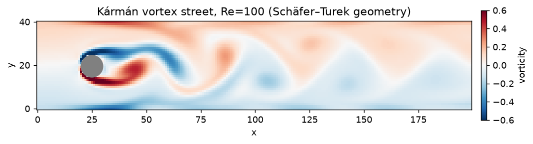
The shedding signal and the Strouhal number
The cross-flow velocity at the wake probe oscillates periodically once the limit cycle is reached. Its power spectrum has a sharp peak at the shedding frequency \(f\), giving \(\mathrm{St} = f D/U_m\).
ts, vs = r["ts"], r["vs"]
mask = ts > ts[-1] * 0.5                          # analyse the developed limit cycle
tt, vv = ts[mask], vs[mask] - vs[mask].mean()
freqs = np.fft.rfftfreq(len(vv), tt[1] - tt[0])
power = np.abs(np.fft.rfft(vv * np.hanning(len(vv))))
f_peak = freqs[1:][np.argmax(power[1:])]
St = f_peak * r["D"] / r["Um"]

fig, (a0, a1) = plt.subplots(1, 2, figsize=(9.2, 3.6))
a0.plot(ts, vs, color=BLUE, lw=0.9)
a0.axvline(ts[-1] * 0.5, color="0.6", ls=":", label="analysis window")
a0.set(xlabel="time", ylabel="wake v", title="shedding signal"); a0.legend(fontsize=8)
a1.plot(freqs, power, color=RED)
a1.axvline(f_peak, color="0.4", ls="--", label=f"f={f_peak:.4f}")
a1.set(xlabel="frequency", ylabel="power", title=f"spectrum → St={St:.3f}", xlim=(0, 8 * f_peak))
a1.legend(fontsize=8)
fig.tight_layout()
plt.show()

print(f"Strouhal number St = {St:.3f}   (Schäfer–Turek 2D-2 benchmark ≈ 0.30)")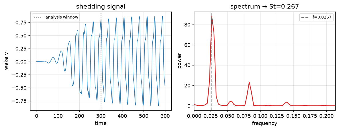
Strouhal number St = 0.267 (Schäfer–Turek 2D-2 benchmark ≈ 0.30)How it compares
| quantity | this run (D=10, CPU) | Schäfer–Turek 2D-2 |
|---|---|---|
| Strouhal \(\mathrm{St}\) | 0.27 (computed here) | 0.295–0.305 |
| \(\Delta p\) across cylinder | ≈2.5 (separate check) | 2.46–2.50 |
| \(C_D\), \(C_L\) | not computed (see note) | 3.22–3.24, ±0.99 |
The Strouhal number lands about 10% below the benchmark. That is the resolution: at \(D=10\) cells the cylinder boundary layer is only ~1 cell thick, which thickens the shed shear layers and lowers the shedding frequency. Refining to \(D\gtrsim30\) (a GPU build) converges \(\mathrm{St}\) toward \(0.30\). The pressure difference, a more forgiving integral quantity, already matches the benchmark well.
NoteDrag and lift coefficients
\(C_D\) and \(C_L\) require integrating the traction over the cylinder surface, which needs a force-on-solid query peclet.flow does not yet expose. Once it does, this example will report the full benchmark set. The Strouhal number (a frequency, from a wake probe) and \(\Delta p\) (from the pressure field) need no force integration.
Adapt this yourself
- Resolve it properly. Raise
D(and the grid with it) on a GPU build to converge the Strouhal number to the benchmark — and dropdt. - Sweep Reynolds. Below
Re≈47the wake is steady (no shedding); above it,Strises gently withRe(the Williamson curve for an unconfined cylinder). - Try other bodies. Swap the SDF for a square cylinder or an aerofoil — the shedding and its frequency change with the separation geometry.
Reproduce this
pip install peclet            # needs peclet-flow >= 0.2.1 (inflow/outflow + backflow + deferred correction)
quarto render examples/cylinder-vortex-street/index.qmd --execute   # compute-heavy (~1 h on CPU)
# ...or against a local source build:
PECLET_LOCAL_BUILD=/path/to/suite/flow/build_mpi OMP_NUM_THREADS=6 \
  quarto render examples/cylinder-vortex-street/index.qmd --execute