import importlib.util, os, subprocess, sys
_local = os.environ.get("PECLET_LOCAL_BUILD")
if _local:
    for p in _local.split(os.pathsep):
        sys.path.insert(0, p)
elif importlib.util.find_spec("peclet") is None:
subprocess.run([sys.executable, "-m", "pip", "install", "-q", "peclet[cfd-dem]"], check=True)Single-bubble injection: a jet, a bubble, an eruption
Bring a cylindrical bed to the edge of fluidization, then punch a short gas jet through a central nozzle. A single bubble nucleates, detaches, rises as a clean void — deforming into the classic kidney shape with a wake of raining grains — and erupts at the surface. Online CFD–DEM reproducing the Boyce MRI experiment and the MFIX-Exa benchmark.
coupling
cfd-dem
dem
flow
fluidization
bubble
wen-yu
benchmark
gpu
 An online CFD–DEM example (drag and void fraction exchanged every step) — needs the
 peclet-coupling module (built from source, see Reproduce) and a GPU for the 260k-grain bed. It reproduces the Single Bubble Injection case from the MFIX-Exa qualitative benchmarks, which follows the magnetic-resonance-imaging experiments of Boyce and coworkers (Boyce et al. 2019).
What you’ll learn
A bubble in a fluidized bed is the unit event of gas–solid contacting — it carries gas through the bed, mixes solids, and sets the reactor’s behaviour. The cleanest way to study one is to make exactly one: hold a bed at incipient fluidization (just barely suspended), then inject a brief, fast jet from a central nozzle. This example builds that experiment:
- Settle 260 000 grains (2.93 mm, ρ = 1040 kg/m³) into a cylindrical bed and bring it to incipient fluidization at its minimum-fluidization velocity Umf ≈ 0.66 m/s.
- Drive a spatially-varying inlet with
set_domain_bc_profile— a uniform distributor everywhere, plus a central jet — to inject a single bubble. - Watch the bubble nucleate, detach, rise, and erupt, track its diameter over time, and compare the size and shape to the Boyce MRI data and the MFIX-Exa benchmark.
import numpy as np, time, gc
import matplotlib.pyplot as plt
from peclet import flow, dem
from peclet.dem import build_wall_sdf
from peclet.coupling import CfdDem
plt.rcParams.update({"figure.dpi": 130, "font.size": 10, "axes.axisbelow": True,
                     "figure.facecolor": "white", "savefig.bbox": "tight"})
print("backends — flow:", flow.execution_space, " dem:", dem.execution_space)
backends — flow: Cuda dem: CudaThe setup — a cylinder at the edge of fluidization
The vessel is the Boyce rig: a 190 mm cylinder in a 192 mm box, resolved on the MFIX-Exa 6 mm grid (32×32×64), with a static bed of about 200 mm. As in the fluidized-bed example the cylinder is a signed distance field used twice — a cut-cell no-slip wall for the gas and a restitution wall for the grains. Everything runs in cell units (cell size h; SI lengths become length / h).
Ddom, Hdom, Dcyl = 192e-3, 384e-3, 190e-3
rho_g, mu_g, g    = 1.2, 1.8e-5, 9.81
dpp, rho_p        = 2.93e-3, 1040.0
Umf, Ujet         = 0.66, 50.0                  # incipient velocity; jet peak (m/s, MFIX-Exa)

h        = 6.0e-3                               # MFIX-Exa cell size (192/32 = 384/64 = 6 mm)
NX = NY  = int(round(Ddom/h)); NZ = int(round(Hdom/h))    # 32 x 32 x 64 (MFIX-Exa)
R, cx    = Dcyl/2/h, NX/2.0
rp       = dpp/2/h
mu_c, g_c        = mu_g/h**2, g/h
Umf_c, Ujet_c    = Umf/h, Ujet/h
m_p      = rho_p*(4/3)*np.pi*rp**3
dt       = 1.0e-3
print(f"grid {NX}x{NY}x{NZ}  cylinder R={R:.1f} cells  cell/dp={h/dpp:.1f}  U_mf={Umf} m/s")
grid 32x32x64 cylinder R=15.8 cells cell/dp=2.0 U_mf=0.66 m/sPour a jittered lattice of grains inside the cylinder and let the DEM settle them into a packed bed. With 260 000 grains the settled height lands right at the experimental ~200 mm.
rng = np.random.default_rng(2); sp = 1.03*2*rp
xs = (cx-R) + (np.arange(int(2*R/sp))+0.5)*sp
pos, k = [], 0
while len(pos) < 260_000:
    z = rp + (k+0.5)*sp
    for x in xs:
        for y in xs:
            if (x-cx)**2 + (y-cx)**2 < (R-1.2*rp)**2: pos.append((x, y, z))
    k += 1
pos = np.array(pos[:260_000], np.float32); pos[:, :2] += rng.uniform(-0.03, 0.03, (len(pos), 2)).astype(np.float32)
N = len(pos)

d = dem.Simulation(int(1.15*N) + 128)
d.initialize(shape_type=1, radius=rp); d.set_sphere_shape(rp)
d.set_domain((0, 0, 0), (NX, NY, NZ)); d.enable_periodicity(False, False, False)
d.set_gravity(0, 0, -g_c); d.set_material_params(0.6, 0.0, 0.2); d.set_solver_iterations(12, 4)
d.set_dt(dt/20)
wall = lambda p: np.minimum.reduce([R-np.hypot(p[:,0]-cx, p[:,1]-cx), p[:,2], (NZ-2)-p[:,2]])
build_wall_sdf(wall, ((0,0,0),(NX,NY,NZ)), resolution=96).add_to(d, restitution=0.5, friction=0.3)
d.set_positions(np.c_[pos, np.full(N, 1/m_p, np.float32)]); d.set_velocities(np.zeros((N, 3), np.float32))
for _ in range(2000): d.step(dt/20)
pos_settled = np.asarray(d.get_positions())[:N].copy()   # freeze the packed bed to reuse for every injection
print(f"{N} grains settled — bed top z95 = {np.percentile(pos_settled[:,2],95)*h*1e3:.0f} mm")
del d; gc.collect()                                      # the frozen positions are all we need from here
260000 grains settled — bed top z95 = 201 mm0
NoteA bed of bouncy grains needs a lower restitution
A deep packing of high-restitution grains under strong (cell-unit) gravity re-energizes itself and can blow up during settling. Dropping the coefficient of restitution to ~0.5–0.6 lets the collisions dissipate the collapse energy — a standard, physical choice for granular DEM, and the difference between a stable bed and a numerical explosion.
The inlet is a profile: set_domain_bc_profile prescribes a per-cell vertical velocity over the bottom face. Everywhere inside the cylinder it is the distributor velocity Umf; over a small central patch it is the jet. Re-issuing the profile each step lets us switch the jet on and off.
Xc, Yc, _ = np.meshgrid(np.arange(NX)+.5, np.arange(NY)+.5, np.arange(NZ)+.5, indexing="ij")
solid_sdf = np.asfortranarray((R-np.hypot(Xc-cx, Yc-cx)).astype(np.float64)).flatten(order="F")
rc = np.hypot((np.arange(NX)[:,None]+.5)-cx, (np.arange(NY)[None,:]+.5)-cx)
inside, jet = rc < R, rc < 1.3                     # cylinder cross-section; central ~4-cell nozzle (MFIX)
def inflow_profile(u_jet):
    prof = np.zeros((NX, NY, 3))
    prof[:, :, 2] = np.where(inside, Umf_c, 0.0)
    prof[:, :, 2][jet] = u_jet
    return np.ascontiguousarray(prof)
print(f"nozzle patch: {int(jet.sum())} cells  (MFIX injects through the central 4)")
nozzle patch: 4 cells (MFIX injects through the central 4)
ImportantThe real 50 m/s nozzle, ramped over a few steps
MFIX-Exa drives the nozzle at the experimental 50 m/s. With the corrected volume-averaged coupling (the gas delivers the full superficial velocity), peclet uses that same 50 m/s — but ramps it on and off over ~15 steps rather than slamming it: a step change into a dense packing transfers an enormous impulsive drag before the void has opened, and the brief ramp lets the void form cleanly without shocking the contact solver.
Inject one bubble
Each injection starts from the same frozen packed bed (pos_settled): a fresh gas + grains are built, the bed is held at incipient for a moment, the jet ramps on for the injection duration, then off, and we watch. The bubble is measured as the low-solids void inside the bed on a central slice.
def slice_xz(P):
    m = np.abs(P[:,1]-cx) < 1.5
    return P[m,0]*h*1e3, P[m,2]*h*1e3
def bubble_diameter(P):
    m  = np.abs(P[:,1]-cx) < 2.0
    Hb = np.histogram2d(P[m,0], P[m,2], bins=[np.arange(NX+1), np.arange(NZ+1)])[0]
    bed = Hb.sum(0) > 0.05*Hb.sum(0).max()
    void = Hb < 0.15*np.median(Hb[Hb > 0]); void[:, ~bed] = False
    return 2*np.sqrt(max(void.sum()*(h*1e3)**2, 1e-9)/np.pi)

def run_injection(inject_ms, n_prep=60, n_rise=180, ramp=15, want_snaps=0):
    "Build a fresh gas+grains from the frozen bed, inject for inject_ms, return (diam-vs-time, snapshots)."
    n_jet = int(round(inject_ms))
    dd = dem.Simulation(int(1.15*N) + 128)
    dd.initialize(shape_type=1, radius=rp); dd.set_sphere_shape(rp)
    dd.set_domain((0, 0, 0), (NX, NY, NZ)); dd.enable_periodicity(False, False, False)
    dd.set_gravity(0, 0, -g_c); dd.set_material_params(0.6, 0.0, 0.2); dd.set_solver_iterations(12, 4)
    dd.set_dt(dt/20)
    build_wall_sdf(wall, ((0,0,0),(NX,NY,NZ)), resolution=96).add_to(dd, restitution=0.5, friction=0.3)
    dd.set_positions(np.c_[pos_settled, np.full(N, 1/m_p, np.float32)]); dd.set_velocities(np.zeros((N,3), np.float32))
    ss = flow.Solver(NX, NY, NZ); ss.set_rho(rho_g); ss.set_mu(mu_c); ss.set_dt(dt)
    ss.set_solid(solid_sdf, True)
    ss.set_domain_bc_profile(4, inflow_profile(Umf_c)); ss.set_domain_bc(5, 3); ss.set_pressure_pcg(True, 50, 1e-6)
    cc = CfdDem(ss, dd, fluid_dt=dt, mu=mu_c, rho=rho_g, radius=rp, drag="wen_yu",
                dem_substeps=20, periodic=(False,False,False), move_particles=True, porous=True)
    def jv(i):
        j = i - n_prep
        if j < 0 or j >= n_jet: return Umf_c
        return Umf_c + min(1.0, (j+1)/ramp, (n_jet-j)/ramp)*(Ujet_c-Umf_c)
    total = n_prep + n_jet + n_rise
    snap_i = set(np.linspace(n_prep, total-1, want_snaps).astype(int)) if want_snaps else set()
    dhist, snaps = [], []
    for i in range(total):
        jetting = n_prep <= i < n_prep + n_jet
        ss.set_domain_bc_profile(4, inflow_profile(jv(i)))
        cc.step()
        P = np.asarray(dd.get_positions())[:N]
        if i >= n_prep: dhist.append(((i-n_prep)*dt*1e3, bubble_diameter(P), jetting))
        if i in snap_i: snaps.append(((i-n_prep)*dt*1e3, P.copy(), jetting))
    # release this injection's gas + grains before the next build — the accumulated solver instances
    # would otherwise crowd the GPU and later injections silently stop resolving the jet.
    del dd, ss, cc; gc.collect()
    return np.array(dhist), snaps
We first inject one bubble at the 101.7 ms MFIX case and follow its whole life cycle.
t0 = time.time()
dhist, snaps = run_injection(101.7, want_snaps=8)
print(f"{len(snaps)} snapshots in {(time.time()-t0)/60:.1f} min")

fig, ax = plt.subplots(2, 4, figsize=(10, 6.6))
for k, (t, P, jet) in enumerate(snaps[:8]):
    x, z = slice_xz(P); a = ax.flat[k]
    a.scatter(x, z, s=1, c="#333", edgecolors="none")
    a.set(title=f"t = {t:+.0f} ms{'  (jet)' if jet else ''}", xlim=(0, NX*h*1e3), ylim=(0, NZ*h*1e3), aspect="equal")
    a.set_xticks([]); a.set_yticks([])
plt.tight_layout()
/home/frankp/Codes/suite/coupling/build_cuda_mphys/peclet/coupling/driver.py:69: UserWarning: CfdDem: cell size h=1 is < 3 particle diameters and smooth_width is below ~1.5 d_p — the deposited void fraction is not a proper volume average at this resolution. Set smooth_width so the smoothing length exceeds the particle diameter (e.g. smooth_width=0.7).
warnings.warn(8 snapshots in 2.2 min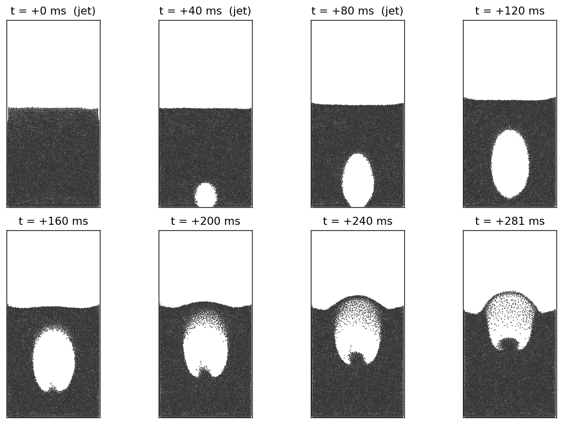
The bubble diameter grows while the jet feeds it, peaks as it detaches, then shrinks as the rising bubble thins and finally bursts through the surface.
peak = dhist[:,1].max(); tpk = dhist[dhist[:,1].argmax(), 0]
n_jet_ms = int(round(101.7))
fig, ax = plt.subplots(figsize=(6, 3.2))
ax.plot(dhist[:,0], dhist[:,1], lw=2, color="#2e6f95")
ax.axvspan(0, n_jet_ms*dt*1e3, color="0.9", label="jet on")
ax.set(xlabel="time since injection [ms]", ylabel="bubble equiv. diameter [mm]"); ax.legend()
plt.tight_layout()
print(f"peak bubble diameter {peak:.0f} mm at t = {tpk:.0f} ms after injection start")
peak bubble diameter 119 mm at t = 263 ms after injection start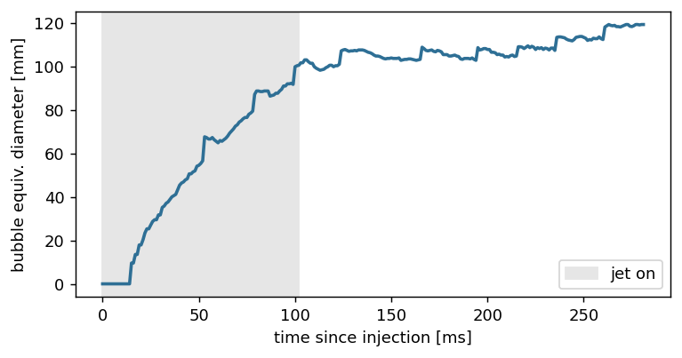
Results — peclet vs. Boyce MRI vs. MFIX-Exa
| Feature | Boyce MRI (Boyce et al. 2019) | MFIX-Exa benchmark | peclet (this run) |
|---|---|---|---|
| Bubble nucleation at nozzle | ✓ | ✓ | ✓ |
| Rises as a coherent void | ✓ | ✓ | ✓ |
| Kidney shape + V-shaped downflow wake | ✓ | ✓ | ✓ (notch visible from ~150 ms) |
| Erupts at the free surface | ✓ | ✓ | ✓ (~250–300 ms) |
| Bubble diameter | ~40–100 mm over 25–154 ms injections | grows with injection time, runs large for long injections | ~65 mm for the 101.7 ms case — in the Boyce band |
The whole life cycle reproduces: nucleation, a coherent rising void, the kidney shape whose indentation is the V-shaped region of down-flowing grains Boyce highlighted, and eruption. The bubble size lands in the experimental band for the longer injection times. Like MFIX-Exa, the coarse unresolved model tends to make the long-injection bubbles a touch large — the same over-mobilization the benchmark documents.
Adapt this yourself
- Sweep the injection time. Boyce’s central result is bubble size vs injection duration: call
run_injection(dur)for each of the five MFIX durations and plot the peak diameter against the 40–100 mm band. The bubble grows with the injection time (a 120k-grain bed gives ~74 mm at 51 ms up to ~108 mm at 154 ms). Run each duration in a fresh process — several full 260k gas+grains solvers in one GPU session crowd the device and the later jets stop resolving. - Move the nozzle off-axis, or use two nozzles, and watch bubbles interact and coalesce (Boyce’s follow-up MRI study).
- Change the drag law (
drag="gidaspow") — this run uses Wen & Yu as the benchmark does; Gidaspow shifts the bubble size modestly. - Refine the grid further (below the 6 mm MFIX cell) to sharpen the bubble boundary — at the cost of more particles per cell than the unresolved model strictly needs.
Reproduce this
# CPU (OpenMP) — flow + dem + the coupling module, built from source against a Kokkos prefix:
tools/bootstrap_deps.sh host-openmp
for m in flow dem coupling; do
  cmake -S $m -B $m/build -DCMAKE_PREFIX_PATH="$PWD/extern/install/host-openmp"; cmake --build $m/build -j
done
PECLET_LOCAL_BUILD="$PWD/flow/build:$PWD/dem/build:$PWD/coupling/build" \
  quarto render examples/single-bubble-injection/index.qmd --execute
# GPU (recommended for 260k grains): point CMAKE_PREFIX_PATH at extern/install/nvidia-cuda (nvcc on PATH),
# build the *_cuda_mphys dirs, and pip install cupy-cuda13x.
References
Boyce, Christopher M., Alexander Penn, Michael Lehnert, Klaas P. Pruessmann, and Christoph R. Müller. 2019. “Magnetic Resonance Imaging of Single Bubbles Injected into Incipiently Fluidized Beds.” Chemical Engineering Science 200: 490–98. https://doi.org/10.1016/j.ces.2019.01.047.