import importlib.util, os, subprocess, sys
_local = os.environ.get("PECLET_LOCAL_BUILD")
if _local:
    for p in _local.split(os.pathsep):
        sys.path.insert(0, p)
elif importlib.util.find_spec("peclet") is None:
subprocess.run([sys.executable, "-m", "pip", "install", "-q", "peclet"], check=True)Trickle flow over a sphere packing
Liquid fed onto a wetting packing through a distributor, gas around it, an open outlet below — three VoF rungs composed into one gas–liquid–solid unit cell, with the colour budget closing at the projection floor.
flow
dem
vof
two-phase
wetting
porous-media
multi-method
gpu
 Wants a GPU build: a DEM packing, one \(48\times48\times96\) two-phase run and three on half that grid, each several thousand steps.
What you’ll learn
The other two-phase pages in this gallery each isolate one piece of physics against a closed-form answer. This one composes three of them and lets the answer be a balance:
- cut-cell VoF — the colour field transported through an immersed solid with openness-weighted geometric fluxes;
- a static contact angle on that solid — \(\theta = 60°\), imposed entirely through the colour field inside the grains, with no force added at the wall;
- two-phase open boundaries — a liquid distributor over part of the inlet face, and an outlet that lets liquid and gas leave and lets gas back in wherever the flow reverses.
The case is a trickle-bed unit cell: liquid dripped onto a gravity-settled random packing of spheres, gas around it, gravity down, an open bottom. There is no analytical answer to check against — a rivulet network is not a spherical cap — so what the page gates instead is everything that must hold whatever the physics does:
- The liquid is conserved exactly. Injected, minus what has left, minus what is held in the box, is zero to about one part in \(10^{13}\) of the injected volume — through a solid, through a partially covered inlet and through an outlet, over thousands of fully coupled steps. That identity is the reason to believe the holdup number at all.
- The projection stays healthy. Every run records
last_pressure_iterations()against its cap and the non-mutatingmax_open_divergence_projected(); a capped run would be discarded, not quoted. No run below reaches its iteration cap — the count is printed with each one — and the divergence of the projected field at the outlet stays below \(10^{-8}\), four to five orders better than the same case gave before the variable-density outflow operator was fixed. - The functionals are followed from a dry bed, in the three quantities a trickle bed is designed around — liquid holdup, wetted-area fraction, pressure drop. They are still rising when the run stops: the liquid load chosen here fills the bed faster than its films drain it, so within the run length this page can afford on a shared GPU the unit cell never reaches the state where the outlet returns what the distributor delivers. That is reported rather than hidden, and it is what makes the run-to-run comparisons below same-time comparisons rather than steady-state ones.
And the honest part, three times over: the Bond number here is the physical one but the Capillary number is set by the grid and is two to three orders too high — an inequality with a proof, in resolution and limits; the run is a filling transient, not a steady state; and at density ratio 1000 the run still conserves and still converges, but the solver’s own gates say the velocities in thin liquid structures are not yet trustworthy there. All three are stated where the numbers are.
The problem: a trickle-bed unit cell
A trickle-bed reactor is a packed column with liquid running down over the grains as films and rivulets while gas occupies the rest of the pore space. The quantities it is designed around are the liquid holdup (how much liquid the bed retains), the wetted fraction (how much of the catalyst surface the liquid actually touches — the rest of it is doing nothing) and the pressure drop. All three are emergent: they come out of a competition between gravity, viscosity and capillarity on a geometry nobody controls in detail.
Three dimensionless groups fix that competition. With \(d_p\) the sphere diameter, \(\delta\) a film thickness, \(\Delta\rho\) the density difference and \(u\) the film surface speed,
\[ \mathrm{Bo} = \frac{\Delta\rho\, g\, d_p^2}{\sigma}, \qquad \mathrm{Ca} = \frac{\mu_\ell u}{\sigma}, \qquad \mathrm{Re}_f = \frac{\rho_\ell u \delta}{\mu_\ell} . \tag{1}\]
\(\mathrm{Bo}\) says whether liquid hanging off a grain falls or stays; \(\mathrm{Ca}\) says whether the film shape is set by capillarity or by shear; \(\mathrm{Re}_f\) says the film is laminar. Water and air on 3 mm packing give \(\mathrm{Bo}\approx 1.2\), which is the number this page matches. It cannot match \(\mathrm{Ca}\), and the reason is a grid statement rather than a modelling one — see resolution and limits.
The film scale itself is a Nusselt balance: a film of thickness \(\delta\) draining down a vertical wall under a body force \(\Delta\rho g\) has
\[ u(\xi) = \frac{\Delta\rho\, g}{\mu_\ell}\left(\delta \xi - \tfrac12 \xi^2\right), \qquad u_{\max} = \frac{\Delta\rho\, g\, \delta^2}{2\mu_\ell}, \tag{2}\]
and \(u_{\max}\) is the speed the distributor is fed at, so that liquid arrives at about the rate a film can carry it away. (peclet reproduces Equation 2 to +0.21 % in flow rate at density ratios 100 and 1000 on a flat wall with an open inlet and an open outlet; that gate is what made this page possible, and it exercises exactly the machinery below.)
What the boundaries have to do
The inlet and outlet are where a two-phase open-boundary problem is won or lost, so they get stated explicitly rather than left to a default.
- Inlet (top). The velocity profile (
set_domain_bc_profile) says how fast fluid enters at each position on the face; the colour profile (set_vof_inflow_profile) says whether what enters there is liquid or gas. A distributor is exactly that pair: a central disc carries \(C=1\) at the Nusselt speed, the rest of the face carries \(C=0\). The flux through a face whose donor cell lies outside the domain is the algebraic \(C_{\text{ghost}}\,a\), never a reconstructed PLIC slab — a prescribed uniform ghost band has no interface in it to reconstruct, and a fractional inflow colour is a statement about the incoming flux, not about a sub-cell interface position. - Outlet (bottom,
set_vof_backflow(4, 0.0)). Zero-gradient where the flow leaves; where the boundary face velocity points back into the domain, the ghost band carries the prescribed backflow colour — here \(0\), gas. That is OpenFOAM’sinletOutletswitch (Rusche 2002), and it is the volume-of-fluid half of the energy-stable two-phase open boundary of Dong (Dong 2014; Dong and Wang 2016), whose backflow term is likewise active only where \(\mathbf{n}\cdot\mathbf{u} < 0\). Without it, a bed that momentarily pushes fluid back through the outlet would draw liquid in and quietly invent volume. - Sides: periodic. This is a unit cell of the interior of a bed, not a laboratory column. A column wall would add its own wetting film and the wall channelling that trickle-bed experimentalists spend their lives avoiding; both are real, neither is what this page measures. (If you do want column walls, model them as an SDF slab and put them at a quarter-integer coordinate — a flat SDF wall at \(k+\tfrac12\) closes the wall cell’s tangential faces and freezes the contact line, as the droplet wetting page measures. The spheres here are curved, so none of their faces sits on the zero level by construction.)
The direct precedent for the configuration is the TU/e coupled immersed-boundary + volume-of-fluid line (Patel et al. 2017) — a static contact angle on resolved particles inside a VoF solver — and, for the physics the page shows, the packed-bed liquid-spreading study of Ambekar, Rüde and Buwa (Ambekar et al. 2022).
import math, time
import numpy as np
import matplotlib.pyplot as plt
from peclet import dem, flow

plt.rcParams.update({"figure.dpi": 130, "font.size": 10, "axes.grid": True,
                     "grid.alpha": 0.3, "axes.axisbelow": True,
                     "figure.facecolor": "white", "savefig.bbox": "tight"})
BLUE, RED, GREY, GREEN, ORANGE = "#1f77b4", "#d62728", "0.80", "#2ca02c", "#ff7f0e"
PRESS_CAP = 600
1. The packing: peclet.dem → an SDF
Same idea as the random packed bed page, with one change: the box is periodic in \(x\) and \(y\) only and a flat SDF floor closes it below, so the grains settle under gravity into a real bed instead of jamming in a triply periodic box. That gives the unit cell what it needs — a rough top surface for the liquid to land on, and a bottom it can drip off.
def settle_bed(N=34, R=7.7, L=48.0, H=260.0, seed=5, dt=0.004, fall=9000, quench=4000):
    """A gravity-settled random packing of N spheres in a laterally periodic column."""
    from peclet.dem import build_wall_sdf
    rng = np.random.default_rng(seed)
    s = dem.Simulation(N)
    s.initialize(shape_type=1, radius=R)
    s.set_domain((0.0, 0.0, -R), (L, L, H))
    s.enable_periodicity(True, True, False)          # periodic sides, a floor below
    s.set_gravity(0.0, 0.0, -9.81)
    s.set_material_params(0.1, 0.0, 0.35)            # restitution, cohesion, friction
    s.set_solver_iterations(24, 8)
    build_wall_sdf(lambda p: p[:, 2], ((0.0, 0.0, -R), (L, L, H)), resolution=32) \
        .add_to(s, restitution=0.1, friction=0.35)   # the floor: positive above z = 0
    pos = np.zeros((N, 4), np.float32)
    pos[:, 0] = rng.uniform(0, L, N); pos[:, 1] = rng.uniform(0, L, N)
    pos[:, 2] = rng.permutation(np.linspace(R + 2, R + 2 + 4.0 * L, N)) + rng.normal(0, 2, N)
    pos[:, 3] = 1.0                                  # inverse mass
    s.set_positions(pos)
    s.set_velocities(np.zeros((N, 3), np.float32))
    for _ in range(fall):
        s.step(dt)
    # A zero-restitution quench alone does not come to rest: a grain that lands on top of the pile
    # keeps rolling, and the packing is then reported with a residual velocity of order 1. Draining
    # the kinetic energy directly -- zero the velocities, step, repeat -- turns the tail of the
    # quench into pure position relaxation, and makes the settled POROSITY reproducible even though
    # the GPU contact solve is not bit-reproducible (float atomics in the contact sum).
    s.set_material_params(0.0, 0.0, 0.35)            # quench into the rigid contact network
    zero = np.zeros((N, 3), np.float32)
    for k in range(quench):
        if k % 400 == 0 or k > quench - 200:
            s.set_velocities(zero)
        s.step(dt)
    p = s.get_positions()[:, :3].astype(float)
    p[:, 2] -= p[:, 2].min() - R                     # rest the lowest grain on z = 0
    # the velocity ONE step regenerates from rest: a measure of the residual unbalanced force
    return p, float(np.abs(s.get_velocities()).max())

t0 = time.time()
POS, VREST = settle_bed()
L48, R48 = 48.0, 7.7
HBED = POS[:, 2].max() + R48
PHI = len(POS) * (4 / 3) * math.pi * R48 ** 3 / (L48 * L48 * HBED)
print(f"{len(POS)} spheres of radius {R48} cells; bed height {HBED:.2f} cells, "
      f"solid fraction {PHI:.3f} (porosity {1 - PHI:.3f})")
print(f"velocity regenerated by one step from rest: {VREST:.1e}   ({time.time() - t0:.0f} s)")
34 spheres of radius 7.7 cells; bed height 51.07 cells, solid fraction 0.553 (porosity 0.447)
velocity regenerated by one step from rest: 4.6e-02 (27 s)Thirty-four equal spheres in a laterally periodic box three diameters wide is a small unit cell, and it shows: the settled bed is partly ordered rather than properly random (the 3-D still below makes this obvious). That is a consequence of the cell size, not of the packing protocol, and it is one of the limits at the end of the page.
Sampling the packing onto the flow grid gives the signed distance field — positive in the fluid, one min over the spheres and their lateral periodic images. Nothing else is solid: no column wall, no floor.
NX, NZ = 48, 96                 # the production grid; halve both for an 8x cheaper preview
ZBED0 = 22.0                    # bed base in cells: 22 below it to drain, ~21 above for the jet

def bed_sdf(nx, nz, pos, R):
    ax = (np.arange(nx) + 0.5)[:, None, None]
    ay = (np.arange(nx) + 0.5)[None, :, None]
    az = (np.arange(nz) + 0.5)[None, None, :]
    best = np.full((nx, nx, nz), 1e30)
    for cx, cy, cz in pos:
        for px in (-nx, 0, nx):                      # lateral periodic images
            for py in (-nx, 0, nx):
                best = np.minimum(best, np.sqrt((ax - (cx + px)) ** 2 + (ay - (cy + py)) ** 2
                                                + (az - cz) ** 2) - R)
    return np.asfortranarray(best)

def place(nx, nz):
    """Scale the DEM packing onto an nx x nx x nz grid and lift it onto the bed base."""
    sc = nx / L48
    p = POS * sc
    p[:, 2] += ZBED0 * (nz / 96.0)
    return p, R48 * sc, ZBED0 * (nz / 96.0), ZBED0 * (nz / 96.0) + HBED * sc
2. The scene
# Solver units: cell size 1, time in seconds. Only the dimensionless groups matter.
RHO_L, MU_L = 100.0, 50.0        # the liquid
MU_RATIO = 50.0                  # water/air is 55; this fixes the gas viscosity at both ratios
BO = 1.2                         # water/air on 3 mm packing: 1.23
THETA = 60.0                     # a wetting solid
DELTA_CELLS = 3.0                # the film thickness the inlet speed is sized on
UMAX_CELLS = 0.3                 # the Nusselt surface speed of that film
RD_CELLS = 8.0                   # distributor radius

def scene(nx, nz, ratio=100.0):
    """Every derived number of the case, at the grid resolution asked for."""
    sc = nx / L48
    pos, R, z0, z1 = place(nx, nz)
    dp = 2 * R                                        # sphere diameter, cells
    rho_g, mu_g = RHO_L / ratio, MU_L / MU_RATIO
    drho = RHO_L - rho_g
    delta, umax = DELTA_CELLS * sc, UMAX_CELLS * sc
    g = 2 * MU_L * umax / (drho * delta ** 2)         # invert eq-nusselt for the body force
    sigma = drho * g * dp ** 2 / BO                   # then fix the Bond number
    return dict(pos=pos, R=R, dp=dp, z0=z0, z1=z1, sc=sc, rho_g=rho_g, mu_g=mu_g, drho=drho,
                delta=delta, umax=umax, g=g, sigma=sigma, rd=RD_CELLS * sc, ratio=ratio,
                Ca=MU_L * umax / sigma, Re_f=RHO_L * umax * delta / MU_L)

S0 = scene(NX, NZ)
print(f"grid {NX}x{NX}x{NZ}   d_p = {S0['dp']:.2f} cells   bed z in "
      f"[{S0['z0']:.1f}, {S0['z1']:.1f}]   distributor radius {S0['rd']:.1f} cells")
print(f"rho_l/rho_g = {RHO_L / S0['rho_g']:.0f}   mu_l/mu_g = {MU_RATIO:.0f}   "
      f"sigma = {S0['sigma']:.4g}   g = {S0['g']:.5g}   u_max = {S0['umax']:.3g} cells/s")
print(f"Bo = {BO}   Ca = {S0['Ca']:.4g}   Re_film = {S0['Re_f']:.3g}   theta = {THETA:.0f} deg")
grid 48x48x96 d_p = 15.40 cells bed z in [22.0, 73.1] distributor radius 8.0 cells
rho_l/rho_g = 100 mu_l/mu_g = 50 sigma = 658.8 g = 0.03367 u_max = 0.3 cells/s
Bo = 1.2 Ca = 0.02277 Re_film = 1.8 theta = 60 deg
ImportantThree settings that are not defaults — and two that now are
set_pressure_fcg is selected after the density closure: set_property_model("rho", ...) fires the solver’s density-mode switch, which reselects the Chebyshev driver and silently discards an earlier choice. On a box with open boundaries at density ratio \(\ge 100\) Chebyshev diverges and MG-PCG burns any cap, while FCG converges — so the order of these two lines is load-bearing. set_pressure_multigrid gets an explicit depth and the velocity solve extra sweeps, as the validated open-boundary channel case does. MG telescoping must stay off: the telescope stage gathers inner cells only, so the outflow face plane does not survive the merge, and the solver refuses the combination outright.
What is a default since the variable-density outflow operator was fixed: the \(1/\rho_f\) outflow correction (set_outflow_rho_correction) and the exact pressure residual, which enable_vof() turns on. Together they are why the outlet divergence below reads \(10^{-9}\) or smaller rather than \(10^{-3}\).
def trickle(nx=NX, nz=NZ, tend=420.0, ratio=100.0, ugas=0.0, probe=50, cap=PRESS_CAP,
            max_steps=18000, snap_fracs=(0.10, 0.25, 0.45, 0.70, 1.00)):
    """One trickle-flow run, to physical time `tend`. `ugas` is the co-current gas inflow as a
    fraction of u_max."""
    P = scene(nx, nz, ratio)
    s = flow.Solver(nx, nx, nz)
    s.set_rho(RHO_L); s.set_mu(MU_L)
    for f in range(4):
        s.set_domain_bc(f, 0, 0, 0, 0)               # periodic sides
    s.set_domain_bc(4, 3, 0, 0, 0)                   # OUTFLOW at the bottom

    xc = (np.arange(nx) + 0.5)[:, None]; yc = (np.arange(nx) + 0.5)[None, :]
    disc = ((xc - nx / 2) ** 2 + (yc - nx / 2) ** 2) < P["rd"] ** 2
    prof = np.zeros((nx, nx, 3))
    prof[:, :, 2] = np.where(disc, -P["umax"], -ugas * P["umax"])
    s.set_domain_bc_profile(5, np.ascontiguousarray(prof))          # the distributor: velocity

    s.set_velocity_solver_params(60)
    s.set_pressure_multigrid(True, levels=6)
    s.set_pressure_solver_params(80)
    s.set_solid(bed_sdf(nx, nz, P["pos"], P["R"]), cutcell_pressure=True)   # the cut-cell IBM
    s.enable_vof()
    s.set_vof(np.zeros((nx, nx, nz), order="F"))                    # the bed starts dry
    s.set_surface_tension(P["sigma"])
    s.set_contact_angle(THETA)                                      # the whole wetting model
    s.set_property_model("rho", "linear", "C", [P["rho_g"], RHO_L - P["rho_g"]])
    s.set_property_model("mu", "linear", "C", [P["mu_g"], MU_L - P["mu_g"]])
    # REDUCED gravity: the force acts on the liquid only, so the gas is exactly force-free and
    # hydrostatic -- which is what a Dirichlet p = 0 outlet assumes. With gravity on the gas too,
    # the outlet accelerates the whole gas column instead of supporting it: a different problem.
    s.set_property_model("force_z", "linear", "C", [0.0, -P["drho"] * P["g"]])
    s.enable_vof_momentum(P["rho_g"], RHO_L)
    s.set_pressure_fcg(True, cap, 1e-11)                            # DRIVER LAST -- see above
    s.set_vof_inflow_profile(5, np.ascontiguousarray(disc.astype(float)))   # ...and its colour
    s.set_vof_backflow(4, 0.0)                                      # gas re-enters on backflow

    eps = np.asarray(s.vof_geometry(0)).copy()          # cell fluid fraction
    cut = (eps > 1e-9) & (eps < 1.0 - 1e-9)             # cells the grain surface passes through
    zc = np.arange(nz) + 0.5
    bed = (zc >= P["z0"]) & (zc <= P["z1"])
    cutbed = cut & bed[None, None, :]
    VB = float(eps[:, :, bed].sum())                    # void volume of the bed
    za = min(nz - 1, int(round(P["z1"] + 2)))                       # pressure probe planes:
    zb = max(0, int(round(P["z0"] - 2)))                            # open planes just off the bed

    dt_cap = 0.5 * s.capillary_dt()
    snap_t = [tend * f for f in snap_fracs]
    hist, snaps = [], {}
    t = 0.0; i = 0
    it_max = capped = 0; div_max = drift = 0.0; b0 = None; cmin, cmax = 1.0, 0.0
    t0 = time.time()
    while t < tend and i < max_steps:
        # dt is re-picked EVERY step from the solver's own two explicit limits. Every ten steps is
        # not enough here: the jet impinging on the bed can double max|u_f| inside ten steps, and
        # the Weymouth-Yue boundedness cap is a hard throw, not a warning.
        lim = s.vof_step_limits()
        dt = min(dt_cap, 0.4 * lim["cfl_dt"]) if lim["cfl_dt"] > 0 else dt_cap
        s.set_dt(dt); s.step(); t += dt; i += 1
        it = s.last_pressure_iterations()
        it_max = max(it_max, it); capped += it >= cap
        want_snap = bool(snap_t) and t >= snap_t[0]
        if i % probe == 0 or want_snap or t >= tend:
            d = s.vof_diagnostics()
            tot = s.vof_bc_volumes_total()              # the ADVECTOR's own boundary fluxes
            b = d["volume"] - sum(tot)
            if b0 is None:
                b0 = b
            drift = max(drift, abs(b - b0))
            cmin, cmax = min(cmin, d["min"]), max(cmax, d["max"])
            div = s.max_open_divergence_projected()     # NON-mutating -- see the note below
            div_max = max(div_max, div)
            C, p = s.get_vof(), np.asarray(s.get_p())
            cd = s.contact_angle_diagnostics()
            hist.append(dict(
                step=i, t=t, dt=dt, iters=it, div=div, drift=drift, volume=d["volume"],
                beta=float((eps[:, :, bed] * C[:, :, bed]).sum()) / VB,     # liquid saturation
                fw=float((C[cutbed] > 0.5).sum()) / max(int(cutbed.sum()), 1),
                dp=float((eps[:, :, za] * p[:, :, za]).sum() / eps[:, :, za].sum()
                         - (eps[:, :, zb] * p[:, :, zb]).sum() / eps[:, :, zb].sum()),
                inflow=tot[5], outflow=-tot[4], solid=d["solid_sum"],
                clipped=d["clipped_volume"], wisps=d["wisps"],
                contact_cells=cd["contact_cells"], apparent=cd["mean_apparent_angle"],
                frame=C[:, nx // 2, :].astype(np.float32).copy()))          # for the movie
            if want_snap:
                snaps[round(snap_t.pop(0), 3)] = C.copy()
    tot = s.vof_bc_volumes_total()
    return dict(P=P, hist=hist, snaps=snaps, eps=eps, cut=cut, cutbed=cutbed, bed=bed, VB=VB,
                C=s.get_vof(), nx=nx, nz=nz, steps=i, ugas=ugas, ratio=ratio, t=t,
                drift=drift, it_max=it_max, capped=capped, div_max=div_max, cap=cap,
                inflow=tot[5], outflow=-tot[4], cmin=cmin, cmax=cmax, wall=time.time() - t0,
                eps_bed=float(eps[:, :, bed].mean()))
Note
max_open_divergence() changes the run; max_open_divergence_projected() does not
The older diagnostic re-imposes the zero-gradient outflow face before measuring, which destroys the projection’s outflow correction — the mechanism by which mass leaves — and then reports the divergence of a field the solver never used. Calling it inside a time loop therefore changes the run, by three to four orders in the budget. On any domain with an outflow face, use the non-mutating sibling, as the driver above does.
3. The run
TEND = 420.0     # physical seconds. The wetting front needs about 300 s to cross
                 # the bed and reach the outlet; the rest is the plateau.
base = trickle(tend=TEND)
print(f"ratio {base['ratio']:.0f}, gas at rest: {base['steps']} steps to t = {base['t']:.0f} s "
      f"({base['wall'] / 60:.0f} min wall)")
print(f"  pressure {base['it_max']}/{base['cap']} iterations, capped steps {base['capped']};  "
      f"max|div(open u)| (projected) {base['div_max']:.2e}")
print(f"  liquid injected {base['inflow']:.6g}, left {base['outflow']:.6g}, "
      f"budget defect {base['drift']:.3e} = {base['drift'] / base['inflow']:.2e} relative")
print(f"  C in [{base['cmin']:.2e}, {base['cmax']:.10f}];  "
      f"colour inside the grains {base['hist'][-1]['solid']:.1e}")
_cl = max(r["clipped"] for r in base["hist"])
print(f"  cut-cell approximation tripwire: worst per-step clipped liquid volume {_cl:.2e} "
      f"({_cl / base['hist'][-1]['volume']:.1e} of the liquid in the box); "
      f"wisp cells {max(r['wisps'] for r in base['hist'])}")
print(f"  contact-angle band at the end: {base['hist'][-1]['contact_cells']} theta cells, "
      f"mean locally measured apparent angle {base['hist'][-1]['apparent']:.1f} deg "
      f"(prescribed {THETA:.0f})")
ratio 100, gas at rest: 9151 steps to t = 420 s (11 min wall)
pressure 38/600 iterations, capped steps 0; max|div(open u)| (projected) 2.05e-09
liquid injected 26208.8, left 6.2262e-24, budget defect 8.860e-10 = 3.38e-14 relative
C in [-4.24e-22, 1.0000000000]; colour inside the grains 0.0e+00
cut-cell approximation tripwire: worst per-step clipped liquid volume 0.00e+00 (0.0e+00 of the liquid in the box); wisp cells 212821
contact-angle band at the end: 5987 theta cells, mean locally measured apparent angle 134.7 deg (prescribed 60)The first thing to check is the one the run cannot fake. Nothing here depends on the physics being right: the budget, the pressure health and the boundedness of \(C\) are properties of the discretisation, and if any of them failed the rest of the page would be void. They do not: the budget closes to 3.4e-14 of the injected volume, the projection uses 38 of its 600 allowed iterations, the outlet divergence sits at 2.1e-09, the colour stays inside \([0, 1]\) (worst excursion 4.2e-22), and the colour inside the grains is exactly zero.
Two lines of that print deserve a note.
The cut-cell tripwire reads zero. clipped_volume measures the one place the cut-cell transport approximates: where the interface crosses a grain wall inside a cell, the PLIC slab is reconstructed on the whole cell and its swept volume multiplied by the face openness, rather than clipped against the solid as well. Over 9151 steps, nothing had to be clipped back into \([0,1]\).
Almost every cell in the box is a wisp. wisps counts cells whose colour is within \(10^{-8}\) of 0 or of 1 without being exactly there — here 212 821 of the 221 184 cells: the round-off wake of a geometric advection scheme, of order \(10^{-20}\) per cell. It is harmless because the wisp guard is on — cells inside that band are treated as pure, so no PLIC normal is ever built from a stencil of \(10^{-20}\) values, which is exactly the degeneracy that takes an emptying domain to NaN. The guard costs nothing in conservation: such a cell is fluxed algebraically at its actual colour, and the budget above is the proof.
keys = sorted(base["snaps"])   # snapshot times
P = base["P"]
sdf_mid = bed_sdf(base["nx"], base["nz"], P["pos"], P["R"])[:, base["nx"] // 2, :]
x = np.arange(base["nx"]) + 0.5
z = np.arange(base["nz"]) + 0.5
fig, axes = plt.subplots(1, len(keys), figsize=(2.05 * len(keys), 4.8), sharey=True)
for ax, k in zip(axes, keys):
    C = base["snaps"][k][:, base["nx"] // 2, :]
    ax.contourf(x, z, np.where((sdf_mid > 0) & (C > 0.02), C, np.nan).T,
                levels=np.linspace(0, 1, 11), cmap="Blues", vmin=0, vmax=1)
    ax.contourf(x, z, (sdf_mid < 0).T.astype(float), levels=[0.5, 1.5], colors=["0.72"])
    for zz in (P["z0"], P["z1"]):
        ax.axhline(zz, color="0.45", lw=0.6, ls=":")
    ax.plot([base["nx"] / 2 - P["rd"], base["nx"] / 2 + P["rd"]], [base["nz"] - 0.4] * 2,
            color=RED, lw=3.5, solid_capstyle="butt")
    h = min(base["hist"], key=lambda r: abs(r["t"] - k))
    ax.set(xlim=(0, base["nx"]), ylim=(0, base["nz"]), aspect="equal",
           title=f"$t = {h['t']:.0f}$ s\n$\\beta = {h['beta']:.3f}$", xlabel="x  [cells]")
    ax.grid(False)
axes[0].set_ylabel("z  [cells]")
plt.show()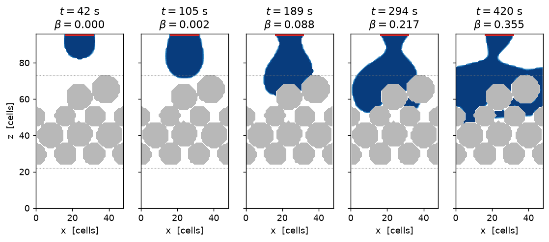
import pyvista as pv
pv.OFF_SCREEN = True

nx, nz = base["nx"], base["nz"]
grid = pv.ImageData(dimensions=(nx, nx, nz), spacing=(1, 1, 1))
grid["sdf"] = bed_sdf(nx, nz, P["pos"], P["R"]).flatten(order="F")
grid["C"] = base["C"].flatten(order="F")
grains = grid.contour([0.0], scalars="sdf")
liquid = grid.contour([0.5], scalars="C")

pl = pv.Plotter(off_screen=True, window_size=(880, 980))
pl.background_color = "white"
pl.add_mesh(grains, color="#bfbfbf", smooth_shading=True)
pl.add_mesh(liquid, color="#2b7bba", opacity=0.95, smooth_shading=True)
pl.camera_position = [(nx * 3.2, -nx * 2.8, nz * 0.95), (nx / 2, nx / 2, nz * 0.48), (0, 0, 1)]
pl.camera.zoom(0.85)
pl.show()
/tmp/ipykernel_1295856/4036978783.py:17: UserWarning: Using static image for notebook display.
Install trame for interactive backends: pip install "pyvista[jupyter]"
pl.show()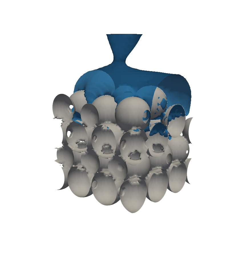
import matplotlib.animation as animation

frames = [r["frame"] for r in base["hist"]]
figm, axm = plt.subplots(figsize=(3.2, 6.0))
axm.contourf(x, z, (sdf_mid < 0).T.astype(float), levels=[0.5, 1.5], colors=["0.72"])
axm.set(xlim=(0, base["nx"]), ylim=(0, base["nz"]), aspect="equal", xlabel="x  [cells]",
        ylabel="z  [cells]")
axm.grid(False)
art = {}

def draw(k):
    for c in art.pop("c", []):
        c.remove()
    cs = axm.contourf(x, z, np.where((sdf_mid > 0) & (frames[k] > 0.02), frames[k], np.nan).T,
                      levels=np.linspace(0, 1, 11), cmap="Blues", vmin=0, vmax=1)
    axm.contourf(x, z, (sdf_mid < 0).T.astype(float), levels=[0.5, 1.5], colors=["0.72"])
    axm.set_title(f"t = {base['hist'][k]['t']:.0f} s")
    art["c"] = cs.collections if hasattr(cs, "collections") else [cs]
    return art["c"]

try:
    anim = animation.FuncAnimation(figm, draw, frames=range(0, len(frames), 2), blit=False)
    anim.save("trickle-flow-packing.mp4", fps=20, dpi=110)
    print(f"wrote trickle-flow-packing.mp4 ({len(frames) // 2} frames)")
except Exception as e:                       # no ffmpeg on the machine rendering the site
    print(f"movie skipped: {e}")
plt.close(figm)
wrote trickle-flow-packing.mp4 (94 frames)4. The colour budget
The geometric transport carries \(\varepsilon_i C_i\) and every flux is the openness-weighted \(o_f F_f\), so the flux sum telescopes exactly and
\[ \sum_i \varepsilon_i C_i(t) \;-\; \int_0^t \! Q_{\text{in}} \,\mathrm{d}t' \;+\; \int_0^t \! Q_{\text{out}} \,\mathrm{d}t' \;=\; \text{const} \tag{3}\]
must hold to round-off, with \(Q_{\text{in}}\) and \(Q_{\text{out}}\) the advector’s own boundary face fluxes (vof_bc_volumes_total()) rather than a re-integration of the velocity field. The floor of the identity is the projection’s divergence residual. This is the strongest statement the page makes, because it holds through a solid, through a partially covered inlet and through an outlet that both loses liquid and takes gas back in — three code paths that only meet in a case like this one.
h = base["hist"]
tt = np.array([r["t"] for r in h])
fig, (a0, a1) = plt.subplots(1, 2, figsize=(9.4, 3.4))
a0.plot(tt, [r["inflow"] for r in h], color=BLUE, lw=1.8, label="injected (distributor)")
a0.plot(tt, [r["outflow"] for r in h], color=RED, lw=1.8, label="left (outlet)")
a0.plot(tt, [r["volume"] for r in h], color=GREEN, lw=1.8, label=r"held: $\sum \varepsilon C$")
a0.plot(tt, [r["inflow"] - r["outflow"] for r in h], "--", color="0.35", lw=1.2,
        label="in $-$ out")
a0.set(xlabel="t  [s]", ylabel="liquid volume  [cells$^3$]", title="the three terms of the budget")
a0.legend(fontsize=8)
a1.semilogy(tt, np.maximum([r["drift"] / max(r["inflow"], 1e-30) for r in h], 1e-18), color=BLUE,
            lw=1.8, label="budget defect / injected")
a1.semilogy(tt, np.maximum([r["div"] for r in h], 1e-18), color=ORANGE, lw=1.4,
            label=r"$\max|\nabla\!\cdot\!(o\,\mathbf{u})|$, projected")
a1.set(xlabel="t  [s]", ylabel="magnitude", title="both at the round-off floor")
a1.legend(fontsize=8, loc="lower right")
plt.show()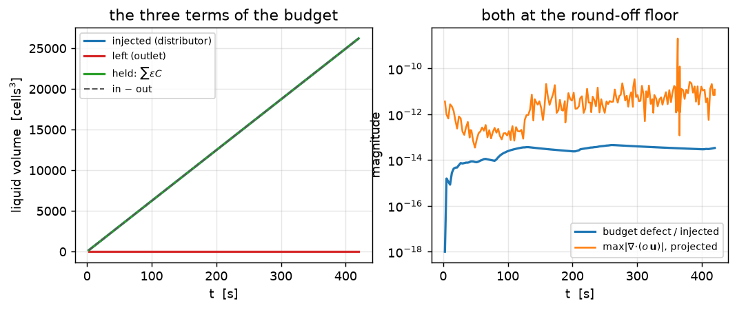
The three curves in the left panel are three independent accountings of the same liquid — the inlet’s own flux ledger, the outlet’s, and a sum over the field — and they close on each other for the whole run. The outlet’s ledger is the flat one: at the end of the run it stands at 6.23e-24, i.e. nothing has left the domain yet — so what the budget is testing here is that a colour field pushed through a partially covered inlet and through a packing loses nothing on the way. The right panel is the statement in one number.
5. Holdup, wetted area, pressure drop
Three functionals, all measured on the bed region (the grains’ bounding slab, dotted in the panels above):
- Liquid saturation \(\beta = \sum_{\text{bed}} \varepsilon C \big/ \sum_{\text{bed}} \varepsilon\) — the fraction of the pore volume the liquid occupies. Multiply by the bed porosity \(\varepsilon_{\text{bed}}\) for the holdup per unit bed volume, the other convention in the literature.
- Wetted fraction \(f_w\) — of the cut cells in the bed (the cells the grain surface passes through), the fraction whose colour is above \(\tfrac12\). It is a proxy for the wetted-area fraction, biased by the cells’ unequal share of surface, and it is quoted as a proxy.
- Pressure drop across the bed: \(\langle p \rangle\) on a plane two cells above the grains minus the same two cells below, each averaged with the cell fluid fraction as the weight. Because the body force acts on the liquid only, this \(\Delta p\) is the frictional drop plus the static head of the liquid the bed is holding, \(\Delta\rho\, g \int \varepsilon C\,\mathrm{d}z\); both are reported.
fig, axes = plt.subplots(1, 3, figsize=(10.8, 3.2))
for ax, key, lab, col in ((axes[0], "beta", r"liquid saturation $\beta$", BLUE),
                          (axes[1], "fw", r"wetted cut-cell fraction $f_w$", GREEN),
                          (axes[2], "dp", r"$\Delta p$ across the bed", RED)):
    ax.plot(tt, [r[key] for r in h], color=col, lw=1.8)
    ax.set(xlabel="t  [s]", ylabel=lab)
axes[2].axhline(0, color="0.5", lw=0.8)
plt.show()

def pct(a, b):
    """Relative change, in per cent, that survives a zero baseline."""
    return (b - a) / abs(a) * 100 if a else float("nan")


def plateau(run, key, frac=0.25):
    hh = run["hist"]; n = max(2, int(len(hh) * frac))
    v = np.array([r[key] for r in hh[-n:]])
    return float(v.mean()), float(v.std())

for k, lab in (("beta", "liquid saturation beta"), ("fw", "wetted cut-cell fraction"),
               ("dp", "pressure drop across the bed")):
    m, sd = plateau(base, k)
    print(f"  {lab:34s} {m:10.4f}  +- {sd:.4f}  (mean +- s.d. over the last quarter)")
BETA, _ = plateau(base, "beta")
DPB, _ = plateau(base, "dp")
HEAD = base["P"]["drho"] * base["P"]["g"] * BETA * base["eps_bed"] * (base["P"]["z1"] - base["P"]["z0"])
print(f"\n  bed porosity {base['eps_bed']:.3f} -> holdup per bed volume "
      f"{BETA * base['eps_bed']:.4f}")
print(f"  static head of that holdup: {HEAD:.3f};  measured Delta p {DPB:.3f};  "
      f"frictional remainder {DPB - HEAD:.3f}")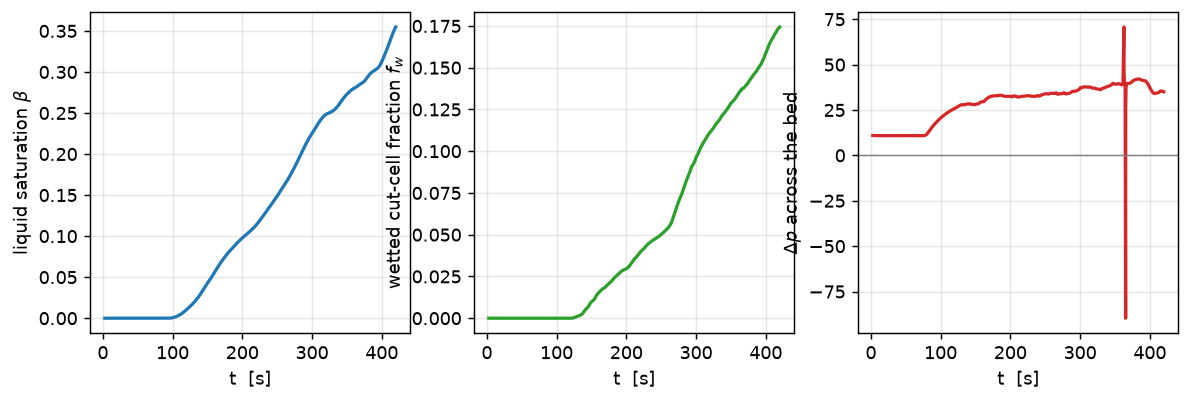
  liquid saturation beta                 0.2982  +- 0.0229  (mean +- s.d. over the last quarter)
  wetted cut-cell fraction               0.1462  +- 0.0135  (mean +- s.d. over the last quarter)
  pressure drop across the bed          34.6544  +- 22.6106  (mean +- s.d. over the last quarter)

  bed porosity 0.443 -> holdup per bed volume 0.1322
  static head of that holdup: 22.511;  measured Delta p 34.654;  frictional remainder 12.144
Read these as filling curves, not plateaus. For the first two minutes or so nothing happens in the bed at all: the liquid hangs from the distributor as a growing pendant body — at this Bond number the disc is below the detachment size, so it does not drip — until it reaches the packing and bridges to it. The front then enters the bed, and the saturation, the wetted fraction and the pressure drop climb together — and they are still climbing when the run stops at \(t =\) 420 s, with nothing returned at the outlet. Two things follow, and both are worth more than a plateau would have been:
- The liquid load is above what this bed drains. The distributor delivers a fixed \(u_{\max}\,\pi r_d^2\); a film of thickness \(\delta\) on a vertical wall carries \(\Delta\rho g \delta^3/3\mu_\ell\) per unit width of wetted contour, and multiplying that by the grain contour a horizontal cut of this packing offers gives a drainage capacity of the same order as the feed. A bed fed at its drainage capacity does not reach a trickle steady state; it accumulates, which is precisely what the curves show and what a trickle-bed operator calls approaching flooding. Reaching a trickle steady state means either a smaller distributor or a much longer run; the second is what the GPU budget for this page did not allow, and the first is the first thing to change if you adapt it.
- The numbers quoted below are therefore levels at a common time, not converged holdups. Since every run on this page is stopped at the same physical time, from the same dry initial condition, on the same packing, the comparisons between them are still controlled — which is what the next three sections use them for.
The wetted fraction climbs with the saturation but stays well below it: the liquid does not spread over the whole grain surface, it selects paths — which is the wetting-efficiency problem the 3-D still shows directly.
One diagnostic in the run print above says the same thing from the wall’s side. The contact-angle band census reports a mean locally measured apparent angle far above the prescribed 60° — the solver imposes 60° on the band, but the angle the interface actually presents while a front is advancing over a dry grain is not the equilibrium angle, and a static model has no term that would make it one. That gap is the honest signature of a moving contact line under a static angle, and closing it is what the dynamic Cox–Voinov rung is for (see the limits).
The same case at half resolution
Three more runs follow — a co-current gas stream, density ratio 1000, and this one — and three \(48\times48\times96\) runs do not fit on a shared GPU. They are therefore run on a grid with every length halved, and this run is the control that makes them readable: the same case as above, so the difference between the two columns is discretisation and nothing else. The sphere diameter drops from 15.4 cells to about 7.7 and the film from three cells to one and a half, while the Bond and Capillary numbers stay exactly where they are — they are built from the scaled lengths. Do not read the two columns as a convergence study: two grids give a difference, not an order, and the difference is the honest error bar.
half = trickle(nx=NX // 2, nz=NZ // 2, tend=TEND)
print(f"half resolution: {half['steps']} steps, pressure {half['it_max']}/{half['cap']}, "
      f"capped {half['capped']}, max|div| {half['div_max']:.2e}, "
      f"budget {half['drift'] / half['inflow']:.2e} relative")
print(f"  {'':20s}{'48 x 48 x 96':>14s}{'24 x 24 x 48':>14s}{'change':>12s}")
for lab, k in (("saturation beta", "beta"), ("wetted fraction", "fw"), ("pressure drop", "dp")):
    a, _ = plateau(base, k); b, _ = plateau(half, k)
    print(f"  {lab:20s}{a:14.4f}{b:14.4f}{pct(a, b):11.1f} %")
half resolution: 5485 steps, pressure 48/600, capped 0, max|div| 8.09e-11, budget 6.49e-14 relative
48 x 48 x 96 24 x 24 x 48 change
saturation beta 0.2982 0.3034 1.7 %
wetted fraction 0.1462 0.1526 4.4 %
pressure drop 34.6544 31.7604 -8.4 %fig, axes = plt.subplots(1, 2, figsize=(7.6, 3.2))
for ax, key, lab in ((axes[0], "beta", r"liquid saturation $\beta$"),
(axes[1], "fw", r"wetted cut-cell fraction $f_w$")):
for run, col, name in ((base, BLUE, f"${NX}^2\\times{NZ}$"),
(half, GREEN, f"${NX // 2}^2\\times{NZ // 2}$")):
ax.plot([r["t"] for r in run["hist"]], [r[key] for r in run["hist"]], color=col, lw=1.7,
label=name)
ax.set(xlabel="t [s]", ylabel=lab)
axes[0].legend(fontsize=8)
plt.show()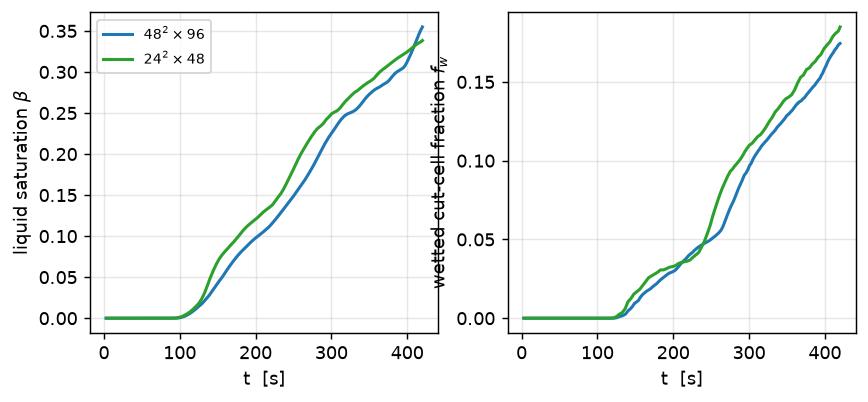
The two grids see the same bed, the same distributor and the same dimensionless numbers, so whatever separates the columns is discretisation. Two mechanisms pull in opposite directions and neither is small: the thinnest structure either grid can carry is about the same number of cells, so the coarse grid’s minimum film is twice as thick in units of the fine grid and tends to hold and spread more liquid; while its throats are resolved by half as many cells, which changes what they cost the flow — and the pressure drop, set by exactly those throats, is the least trustworthy of the three functionals for that reason. Which mechanism wins is not something to read off a single pair of runs. Take the spread as the error bar on every functional here — measured on this run, 2 % on the holdup, 4 % on the wetted fraction and 8 % on the pressure drop.
6. Does a co-current gas stream change anything?
So far the gas has been at rest: the part of the inlet face outside the distributor prescribes zero velocity, so gas moves only because the liquid drags it. A real trickle bed runs gas down the column together with the liquid. The change is one line — the annulus of the inlet profile carries a downward velocity at \(C = 0\) — and everything else, the packing included, is identical. Both columns below are the half-resolution grid, against the control of the previous section.
gas = trickle(nx=NX // 2, nz=NZ // 2, tend=TEND, ugas=0.25)   # a quarter of the liquid speed
print(f"co-current gas at {gas['ugas']:.2f} u_max: pressure {gas['it_max']}/{gas['cap']}, "
      f"capped {gas['capped']}, max|div| {gas['div_max']:.2e}, "
      f"budget {gas['drift'] / gas['inflow']:.2e} relative")
co-current gas at 0.25 u_max: pressure 46/600, capped 0, max|div| 9.96e-11, budget 2.23e-14 relativefig, axes = plt.subplots(1, 3, figsize=(10.8, 3.2))
for ax, key, lab in ((axes[0], "beta", r"$\beta$"), (axes[1], "fw", r"$f_w$"),
(axes[2], "dp", r"$\Delta p$")):
for run, col, name in ((half, BLUE, "gas at rest"), (gas, ORANGE, "co-current gas")):
ax.plot([r["t"] for r in run["hist"]], [r[key] for r in run["hist"]], color=col, lw=1.7,
label=name)
ax.set(xlabel="t [s]", ylabel=lab)
axes[0].legend(fontsize=8)
plt.show()
print(f" {'':20s}{'gas at rest':>14s}{'co-current':>14s}{'change':>12s}")
for k, lab in (("beta", "saturation beta"), ("fw", "wetted fraction"), ("dp", "pressure drop")):
a, _ = plateau(half, k); b, _ = plateau(gas, k)
print(f" {lab:20s}{a:14.4f}{b:14.4f}{pct(a, b):11.1f} %")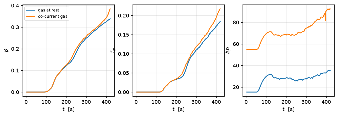
                         gas at rest    co-current      change
  saturation beta             0.3034        0.3252        7.2 %
  wetted fraction             0.1526        0.1765       15.7 %
  pressure drop              31.7604       85.5826      169.5 %
Both signs in that table are the ones trickle-bed correlations give: holdup and pressure drop increase with gas load in the trickle regime, because a co-current stream drags liquid down the column and presses it into the pore space instead of blowing it out. Here the response is very unevenly distributed between the three — the holdup moves by +7 %, the wetted fraction by +16 %, and the pressure drop by +169 % — and the size of that last number is a reminder that at this Capillary number the interfaces are far stiffer than a real bed’s, so the gas has to work much harder to get past them. The pressure solve works harder too (46 iterations against 48 with the gas at rest, both under the cap of 600), and the budget still closes to 2.2e-14 of the injected volume.
7. Density ratio 1000
Water and air are a factor 1000 apart, not 100. Everything so far is at 100, because that is where the solver’s momentum-consistent transport is unambiguously validated. Ratio 1000 is where the honest reporting starts, so it gets its own run — again on the half-resolution grid, against the same control.
r1000 = trickle(nx=NX // 2, nz=NZ // 2, tend=TEND, ratio=1000.0)
print(f"ratio {r1000['ratio']:.0f}: pressure {r1000['it_max']}/{r1000['cap']}, "
      f"capped {r1000['capped']}, max|div| {r1000['div_max']:.2e}")
print(f"  budget defect {r1000['drift'] / r1000['inflow']:.2e} relative, "
      f"C in [{r1000['cmin']:.2e}, {r1000['cmax']:.10f}]")
print(f"  {'':20s}{'ratio 100':>14s}{'ratio 1000':>14s}{'change':>12s}   (both half res)")
for k, lab in (("saturation beta", "beta"), ("wetted fraction", "fw"), ("pressure drop", "dp")):
    a, _ = plateau(half, lab); b, _ = plateau(r1000, lab)
    print(f"  {k:20s}{a:14.4f}{b:14.4f}{pct(a, b):11.1f} %")
ratio 1000: pressure 63/600, capped 0, max|div| 4.78e-11
budget defect 8.22e-14 relative, C in [-2.82e-22, 1.0000000000]
ratio 100 ratio 1000 change (both half res)
saturation beta 0.3034 0.3056 0.7 %
wetted fraction 0.1526 0.1539 0.8 %
pressure drop 31.7604 30.8907 -2.7 %The machinery does not care: the budget closes to 8.2e-14, the colour stays inside \([0, 1]\), the projection converges in 63 of its 600 allowed iterations and the outlet divergence stays at 4.8e-11 — the same four statements as at ratio 100, at ten times the density contrast, on a box with an open inlet and an open outlet, which is the configuration that used to cap every pressure driver whatever it was given.
The functionals themselves move, and by how much is in the table. Do not over-read it in either direction. The bed is stochastic — the DEM packing is not bit-reproducible — and a rivulet network is chaotic, so the spread between two nominally identical configurations is of the same size as the effect being looked for; the two-grid comparison of the previous section is the calibration for that. What licenses or forbids reading physics out of the ratio-1000 column is not this table but the box below.
WarningWhat the solver’s own gates say about ratio 1000 on an open boundary
Two measurements bound the trust to put in the ratio-1000 column. The good one: a Nusselt falling film with an open inlet and an open outlet reproduces the analytical flow rate to +0.21 % at ratio 1000 just as at 100, in 64 pressure iterations, with the outlet divergence at \(2\times10^{-12}\) — so the boundary machinery is sound at that ratio. The bad one: a resting liquid pool with a gas stream blown over it, at the same ratio, loses \(10^{-3}\) of its volume in 500 steps and picks up 3 % of the gas inlet speed where it should pick up nothing. That is a spurious-current / momentum-consistency defect, not an outflow-operator one, and it is the sharpest open two-phase item in the solver. A trickle bed is closer to the second configuration than to the first: the conservation of the ratio-1000 column is exact, the velocities in the thin liquid structures carry that defect, and no quantitative physical claim is made from them here.
8. Resolution and limits
The Capillary number is set by the grid, not by a choice. For a film of thickness \(\delta\) fed at the Nusselt speed on a grain of diameter \(d_p\), Equation 1 and Equation 2 combine into
\[ \mathrm{Ca} \;=\; \frac{\mu_\ell u_{\max}}{\sigma} \;=\; \frac{\mathrm{Bo}}{2}\left(\frac{\delta}{d_p}\right)^{\!2} , \tag{4}\]
with \(\mu_\ell\), \(g\) and \(\sigma\) all cancelling. So once the Bond number is fixed at its physical value, the Capillary number is fixed by one geometric ratio: how thin the film is compared with the grain. A geometric VoF cannot carry a film thinner than about three cells, and the grains here are 15.4 cells across, so the smallest \(\delta/d_p\) this grid can express is about 0.2 — and the Capillary number that goes with it is the 0.023 printed above. A water/air trickle bed runs at \(\delta/d_p \sim 10^{-2}\), i.e. \(\mathrm{Ca}\sim 10^{-4}\) — three orders lower. Recovering those three orders means lowering \(\delta/d_p\) by a factor \(\sim\!30\), i.e. resolving each grain with \(\sim\!500\) cells instead of 15, which costs a factor \(\sim\!3\times10^{4}\) in cells for the same bed. That is the honest scope of this page: the Bond number is physical, the Capillary number is a grid artefact, and no amount of parameter tuning changes that — only resolution does. What the page therefore shows is the structure of trickle flow (films, rivulets, partial wetting, a holdup that saturates) at a Capillary number two to three orders too high, not a predicted holdup for a named system.
The other limits, briefly:
- The contact angle is static. A real rivulet on a grain pins on defects and advances and recedes at different angles, which is what makes rivulets stay where they are. The solver has the Cox–Voinov dynamic angle and advancing/receding hysteresis (
set_contact_angle_dynamic,set_contact_angle_hysteresis), and switching them on is a one-line change to the driver — but a dynamic-wetting result must state its slip length, and calibrating that is a page of its own. - The cut-cell flux is an approximation where the interface crosses a grain. The PLIC polyhedron is reconstructed on the whole cell and its swept volume multiplied by the face openness, rather than clipped against the solid too. It is conservative either way and exact where the interface and the wall are parallel or the cell is whole; where they cross, the distribution of liquid inside that cell is O(1) wrong.
vof_diagnostics()["clipped_volume"]is the tripwire and it is printed with the run above. - The wetted fraction is a cut-cell count, not an area integral. Cells carry unequal shares of the grain surface, so \(f_w\) is a proxy — good for a trend and for comparing two runs on the same packing, not for an absolute wetting efficiency.
- No steady state. Every functional is a level at the end of a fixed-length run on a bed that is still filling (section 5). The comparisons are same-time comparisons on the same packing from the same dry start, which is a controlled experiment; the absolute holdup is not a converged operating point and should not be read against a correlation.
- The bed is partly ordered. 34 equal spheres in a periodic box three diameters wide settle into something closer to a lattice than to a random packing. A random bed’s throat-size distribution is much wider, and it is the narrow throats that decide where liquid goes — so the paths here are cleaner than a real bed’s. Widening the cell is the fix, and it costs cells.
- One packing, one seed. 34 grains is a unit cell, not a statistical sample. Every number here belongs to this bed; the spread over packings is not measured. The DEM packing is also not bit-reproducible — the GPU contact solve sums float contributions atomically — so re-running the first cell gives a slightly different bed.
- Resolution. The half-resolution control in section 5 is the size of the discretisation error to attach to every functional here. It is a control, not a convergence study: two grids give a difference, not an order.
Collocated cross-check
peclet’s cell-centred solver (flow.SolverColocated) runs two-phase flow since rung V8 — variable density in the approximate projection, surface tension as a face acceleration — and the parasitic currents and capillary oscillations pages carry that column.
This page cannot have one, and the reason is the solid. The collocated two-phase path is all-fluid: the openness-weighted cut-cell colour transport, the solid-band fill and the contact-angle plane this page is built on exist on the staggered grid only. The composition is refused rather than silently approximated:
pos32, R32, _, _ = place(32, 32)
sc32 = flow.SolverColocated(32, 32, 32)
sc32.set_rho(1.0); sc32.set_mu(0.1)
sc32.set_solid(bed_sdf(32, 32, pos32, R32), cutcell_pressure=True)   # single-phase: accepted
try:
    sc32.enable_vof()
    print("enable_vof() succeeded")
except RuntimeError as e:
    print(f"enable_vof() raised RuntimeError:\n  {e}")
enable_vof() raised RuntimeError:
enable_vof: geometric VoF on SolverColocated (rung V8) is ALL-FLUID only — an immersed solid needs the cut-cell face acceleration and the matching one-sided closures, which is a later rung. Use the staggered Solver (rung V5a supports cut cells).Every number on this page is a staggered number.
Adapt this yourself
- Change the wettability.
set_contact_angle(120)makes the grains non-wetting, and the liquid should stop filming and start channelling;set_contact_angle_field(theta)takes a per-cell angle, so a partially poisoned catalyst is one array away. This is the cheapest interesting experiment on the page. - Change the distributor. The inlet is two arrays — a velocity profile and a colour profile. Two point sources instead of one central disc, an annulus, a full-face rain: all of them are a change to
discand nothing else. Maldistribution is the geometry of that array. - Change the flow rate.
UMAX_CELLSsets the Nusselt inlet speed; the body force follows from Equation 2 and \(\sigma\) fromBO, so the Capillary number stays put and only the liquid load moves. That sweep is the holdup-versus-flow-rate curve. - Wet the bed first.
set_vof(C0)with a pre-filled pore space and no inflow gives the draining problem — residual holdup — instead of the wetting one. - Put a column wall on it. An SDF slab pair
min-ed into the packing SDF at a quarter-integer coordinate. The sides then stop being periodic, and the wall film and wall channelling appear: the laboratory-column problem rather than the unit cell. - Go multi-rank. The identical script runs under
mpirun -np N python …. The cut-cell colour transport, the contact-angle band fill and the boundary ledger are all decomposition-independent and gated at np = 1/2/4 with the block cut going through the inlet plane, the outlet plane and the packing.
Reproduce this
The compiled solver runs this, so its outputs are frozen into the site. To regenerate:
pip install peclet            # the solver, from PyPI
quarto render examples/trickle-flow-packing/index.qmd --execute
# ...or against a local source build of the suite (GPU):
PECLET_LOCAL_BUILD=/path/to/suite/flow/build_cuda:/path/to/suite/dem/build_cuda \
  OMP_NUM_THREADS=8 OMP_PROC_BIND=false \
  quarto render examples/trickle-flow-packing/index.qmd --execute
The machinery this page composes is gated inside the solver repo by tests/kokkos/test_vof_bc.cpp (the colour budget through an inlet and an outlet, and the composed packing-plus-boundary scene), tests/kokkos/test_vof_cutcell.cpp (conservation through a solid), tests/kokkos/test_vof_wetting.cpp (the contact-angle fill), their MPI twins at np = 1/2/4, and the physics studies tests/study/vof_open_boundaries.py (the Nusselt film and the gas-over-pool case quoted above) and tests/study/vof_wetting.py.
References
Ambekar, Aniket S., Ulrich Rüde, and Vivek V. Buwa. 2022. “Forces Governing the Dynamics of Liquid Spreading in Packed Beds.” Journal of Fluid Mechanics 948: A13. https://doi.org/10.1017/jfm.2022.665.
Dong, S. 2014. “An Outflow Boundary Condition and Algorithm for Incompressible Two-Phase Flows with Phase Field Approach.” Journal of Computational Physics 266: 47–73. https://doi.org/10.1016/j.jcp.2014.02.011.
Dong, Suchuan, and Xiaoyu Wang. 2016. “A Rotational Pressure-Correction Scheme for Incompressible Two-Phase Flows with Open Boundaries.” PLoS ONE 11 (5): e0154565. https://doi.org/10.1371/journal.pone.0154565.
Patel, H. V., S. Das, J. A. M. Kuipers, J. T. Padding, and E. A. J. F. Peters. 2017. “A Coupled Volume of Fluid and Immersed Boundary Method for Simulating 3D Multiphase Flows with Contact Line Dynamics in Complex Geometries.” Chemical Engineering Science 166: 28–41. https://doi.org/10.1016/j.ces.2017.03.012.
Rusche, Henrik. 2002. “Computational Fluid Dynamics of Dispersed Two-Phase Flows at High Phase Fractions.” PhD thesis, Imperial College London.