Non-spherical Stokes drag: exact spheroids, then cubes

Measure a shape’s drag against a sphere of the same volume in the same periodic box, so the box cancels — validated against the exact Oberbeck spheroid solution before it is used to predict anything.

flow

IBM

csg

verification

analytic

drag

GPU

Author

Peclet

Published

August 30, 2026

GPU example — the frozen page reads correctly without a solver.

What you’ll learn

Engineering correlations for non-spherical drag are built on sphericity: one number standing in for a shape. It is worth knowing how well that works, and the only way to find out is to measure shapes whose drag you can also compute exactly.

This page does that in three moves:

Establish the method. Drag in a periodic box is not drag in an unbounded fluid — at solid fraction \(\phi\) the difference is tens of percent. Measuring a shape and an equal-volume sphere in the same box and reporting the ratio makes the leading blockage cancel. That is an assumption, so it gets a ladder.
Validate it against an exact solution. A prolate spheroid’s Stokes drag is known in closed form (Oberbeck 1876; Happel & Brenner §4-26), both along and across its axis. If the ratio method reproduces those, the method is sound.
Then predict. With the method validated, the cube and the spherocylinder become measurements worth quoting, and the sphericity correlations become the thing under test rather than the reference.

Along the way: peclet.core.geom’s leaves differ in whether they are distance-exact (sphere, box, capsule) or only a bound (ellipsoid, superquadric). Whether that matters for a cut-cell solver is an empirical question, and this page answers it.

import importlib.util, os, subprocess, sys
_local = os.environ.get("PECLET_LOCAL_BUILD")
if _local:
    for p in _local.split(os.pathsep):
        sys.path.insert(0, p)
elif importlib.util.find_spec("peclet") is None:
    subprocess.run([sys.executable, "-m", "pip", "install", "-q", "peclet"], check=True)

Requires a recent peclet

peclet.core.geom, the analytic-scene API and hydro_force_torque_reaction are newer than the current PyPI release. The page is frozen and renders regardless.

import time
import numpy as np
import matplotlib.pyplot as plt
from scipy.special import gamma as gamma_fn
from peclet import flow as sdflow
from peclet.core import geom

plt.rcParams.update({"figure.dpi": 130, "font.size": 9, "axes.axisbelow": True,
                     "figure.facecolor": "white", "savefig.bbox": "tight"})

RHO, MU, FBODY = 1.0, 0.1, 1e-4        # cell units: h = 1
RV = 8.0                                # volume-equivalent RADIUS, in cells — fixed across boxes
VOL = 4.0 / 3.0 * np.pi * RV ** 3
KI_I, KI_R = 2, 17

Kokkos::OpenMP::initialize WARNING: OMP_PROC_BIND environment variable not set
  In general, for best performance with OpenMP 4.0 or better set OMP_PROC_BIND=spread and OMP_PLACES=threads
  For best performance with OpenMP 3.1 set OMP_PROC_BIND=true
  For unit testing set OMP_PROC_BIND=false

The method

Hold the body fixed, drive the fluid with a uniform body force \(f\), and read the force on the body from the discrete reaction — the momentum the fluid actually lost to it. Define

\[ \lambda \;=\; \frac{F_{\text{body}}}{6\pi\mu R_v \langle u\rangle}, \tag{1}\]

with \(R_v\) the volume-equivalent radius and \(\langle u\rangle\) the superficial (whole-box) mean velocity. For a sphere this is exactly the simple-cubic array drag ratio Hasimoto (1959) gives in closed form, so the sphere run is a calibration of the whole chain. For any other shape at the same volume, \(K = \lambda_{\text{shape}} / \lambda_{\text{sphere}}\) is the drag correction factor with the box divided out.

_RCACHE = {}
VSOL = {}      # (label, N) -> the solver's own count of SOLID staggered cells

def run(build, n, label, tol=1e-7, dt=1000.0, maxit=3000):
    key = (label, n, tol, dt, maxit)
    if key not in _RCACHE:
        _RCACHE[key] = _run(build, n, label, tol, dt, maxit)
    return _RCACHE[key]

def _run(build, n, label, tol, dt, maxit):
    """Steady Stokes drag on one analytic body in a periodic box, iterated to a steady mean.

    The time step only sets how fast the transient is walked off -- the implicit viscous solve is
    unconditionally stable and the fixed point is dt-independent. That is checked below rather
    than asserted.
    """
    b = geom.SceneBuilder()
    root = build(b)
    ni, nr, _, _ = b.encode()
    inst_ints = np.zeros((1, KI_I), dtype=np.int32); inst_ints[0] = (root, -1)
    inst_reals = np.zeros((1, KI_R))
    inst_reals[0, 0:3] = (0.5 * n,) * 3
    inst_reals[0, 6] = 1.0; inst_reals[0, 7] = 1.0

    s = sdflow.Solver(n, n, n)
    s.set_rho(RHO); s.set_mu(MU); s.set_dt(dt); s.set_advection(False)
    s.set_velocity_solver_params(100); s.set_pressure_solver_params(25)
    s.set_pressure_multigrid(True, levels=4)
    s.set_scene(np.asarray(ni, dtype=np.int32), np.asarray(nr, dtype=float),
                inst_ints.ravel(), inst_reals.ravel(), periodic=True)
    s.set_solid_from_scene(True)
    s.set_body_force(FBODY, 0.0, 0.0)
    nc = s.fluid_momentum_cells()[0]
    prev, it, t0 = 0.0, 0, time.time()
    while it < maxit:
        s.step(); it += 1
        um = float(np.asarray(s.get_u()).sum()) / nc
        if it > 5 and abs(um - prev) < tol * abs(um):
            break
        prev = um
    force = float(np.asarray(s.hydro_force_torque_reaction())[0][0][0])
    lam = force / (6 * np.pi * MU * RV * um)
    VSOL[(label, n)] = n ** 3 - nc
    print("   %-30s N=%3d  lambda=%8.5f   V_solid(discrete)=%7d  (analytic %7.0f)  %4d steps %3.0fs"
          % (label, n, lam, n ** 3 - nc, VOL, it, time.time() - t0))
    return lam

def hasimoto(c):
    """Simple-cubic array drag ratio: Hasimoto (1959) extended by Sangani & Acrivos (1982).

    The two extra terms matter: at c = 0.125 the four-term series gives 4.533 while this one
    gives 4.289, against Zick & Homsy's tabulated 4.292.
    """
    return 1.0 / (1 - 1.7601 * c ** (1 / 3) + c - 1.5593 * c ** 2
                  + 3.9799 * c ** (8 / 3) - 3.0734 * c ** (10 / 3))

The shapes — all at the same volume

AR = 2.0                                   # spheroid aspect ratio
B = RV / AR ** (1 / 3.0); A = AR * B       # prolate semi-axes, equal volume
HC = (VOL / 8.0) ** (1 / 3.0)              # cube half-side, equal volume
# spherocylinder (capsule): radius RC, cylinder half-length LC, volume = pi RC^2 (2 LC) + 4/3 pi RC^3
RC = 0.75 * RV
LC = (VOL - 4 / 3 * np.pi * RC ** 3) / (2 * np.pi * RC ** 2)

def quat_align(a, b):
    """Unit quaternion (x,y,z,w) whose rotation carries the BODY direction a onto the WORLD b."""
    a = np.asarray(a, float); a /= np.linalg.norm(a)
    b = np.asarray(b, float); b /= np.linalg.norm(b)
    axis = np.cross(a, b); c = float(np.dot(a, b))
    if np.linalg.norm(axis) < 1e-12:
        return [0.0, 0.0, 0.0, 1.0] if c > 0 else [1.0, 0.0, 0.0, 0.0]
    axis /= np.linalg.norm(axis); ang = np.arccos(np.clip(c, -1, 1)); h = np.sin(ang / 2)
    return [float(axis[0] * h), float(axis[1] * h), float(axis[2] * h), float(np.cos(ang / 2))]

# a cube BODY DIAGONAL onto the flow direction (+x)
DIAG_Q = quat_align([1.0, 1.0, 1.0], [1.0, 0.0, 0.0])

# Rounded cubes as SUPERQUADRICS. core's leaf is [rx, ry, rz, n] with the implicit
#   |x/rx|^n + |y/ry|^n + |z/rz|^n = 1,
# so n IS the exponent: n = 2 is an ellipsoid and large n approaches a box. The literature
# reference below uses the reciprocal "blockiness" convention e = 2/n (e = 1 sphere, e -> 0
# box), so the two are related by n = 2/e -- a trap worth stating, since both conventions are
# written "e". The superellipsoid volume is
#   V = 8 rx ry rz Gamma(1+1/n)^3 / Gamma(1+3/n),
# which fixes the semi-axis at a given equal-volume radius R_v.
def sq_radius(n, r_v):
    return r_v * ((np.pi / 6) * gamma_fn(1 + 3 / n) / gamma_fn(1 + 1 / n) ** 3) ** (1 / 3.0)

BLOCKINESS = (0.2, 0.4)                      # the reference's e
SQ = {e: (2.0 / e, sq_radius(2.0 / e, RV)) for e in BLOCKINESS}
for e, (n_, r_) in SQ.items():
    print("superquadric  reference e=%.1f  ->  core exponent n=%.2f   equal-volume semi-axis "
          "R=%.4f   (R/d_v = %.5f)" % (e, n_, r_, r_ / (2 * RV)))
print("   convention check: n=2 must give exactly the sphere radius -> %.5f (R_v = %.1f)"
      % (sq_radius(2.0, RV), RV))

SHAPES = {
    "sphere (exact leaf)":        lambda b: b.add_leaf("sphere", [RV]),
    "sphere via ellipsoid leaf":  lambda b: b.add_leaf("ellipsoid", [RV, RV, RV]),
    "prolate AR=2, axial":        lambda b: b.add_leaf("ellipsoid", [A, B, B]),
    "prolate AR=2, broadside":    lambda b: b.add_leaf("ellipsoid", [B, A, B]),
    "cube, face-on":              lambda b: b.add_leaf("box", [HC, HC, HC]),
    # Same cube turned so a body DIAGONAL points along the flow. A cube has cubic symmetry, so
    # its translational resistance tensor must be isotropic and the two must agree -- a symmetry
    # check the solver has no way to satisfy by accident.
    "cube, diagonal-on":          lambda b: b.add_leaf(
        "box", [HC, HC, HC], rotation=DIAG_Q),
    "capsule, axial":             lambda b: b.add_leaf(
        "capsule", [RC, LC], rotation=[0.0, 0.0, float(np.sin(np.pi / 4)),
                                       float(np.cos(np.pi / 4))]),
    "rounded cube e=0.2":         lambda b: b.add_leaf(
        "superquadric", [SQ[0.2][1]] * 3 + [SQ[0.2][0]]),
    "rounded cube e=0.4":         lambda b: b.add_leaf(
        "superquadric", [SQ[0.4][1]] * 3 + [SQ[0.4][0]]),
}
print("R_v = %.2f cells   cube side %.3f   spheroid a=%.3f b=%.3f   capsule r=%.3f L=%.3f"
      % (RV, 2 * HC, A, B, RC, 2 * LC))

superquadric  reference e=0.2  ->  core exponent n=10.00   equal-volume semi-axis R=6.5377   (R/d_v = 0.40860)
superquadric  reference e=0.4  ->  core exponent n=5.00   equal-volume semi-axis R=6.7640   (R/d_v = 0.42275)
   convention check: n=2 must give exactly the sphere radius -> 8.00000 (R_v = 8.0)
R_v = 8.00 cells   cube side 12.896   spheroid a=12.699 b=6.350   capsule r=6.000 L=10.963

capsule is a y-axis primitive, so the axial case rotates it onto x, the flow direction.

N_MAIN = 96                      # the measurement box: phi = 0.0024, dilute enough that
print("N=%d, phi=%.5f" % (N_MAIN, VOL / N_MAIN ** 3))   # the ratio's box terms are small
lam = {k: run(v, N_MAIN, k) for k, v in SHAPES.items()}
phi = VOL / N_MAIN ** 3
# the fixed point must not depend on how we walked to it
lam_slow = run(SHAPES["sphere (exact leaf)"], N_MAIN, "sphere @ dt=200", dt=200.0, maxit=8000)
print("\n   dt-independence of the fixed point: lambda(dt=1000) = %.6f   lambda(dt=200) = %.6f"
      "   -> %.2e relative" % (lam["sphere (exact leaf)"], lam_slow,
                               abs(lam_slow / lam["sphere (exact leaf)"] - 1)))
print("\n   sphere: lambda=%.5f   Hasimoto/Sangani-Acrivos SC = %.5f   (%+.2f%%)"
      % (lam["sphere (exact leaf)"], hasimoto(phi),
         100 * (lam["sphere (exact leaf)"] / hasimoto(phi) - 1)))
print("   sphere authored as an ELLIPSOID leaf (a BOUND, not a distance): %+.3f%% from the "
      "exact-distance sphere leaf" %
      (100 * (lam["sphere via ellipsoid leaf"] / lam["sphere (exact leaf)"] - 1)))

N=96, phi=0.00242
   sphere (exact leaf)            N= 96  lambda= 1.29739   V_solid(discrete)=   2104  (analytic    2145)  1786 steps 143s
   sphere via ellipsoid leaf      N= 96  lambda= 1.29739   V_solid(discrete)=   2104  (analytic    2145)  1786 steps 110s
   prolate AR=2, axial            N= 96  lambda= 1.22030   V_solid(discrete)=   2154  (analytic    2145)  1886 steps 117s
   prolate AR=2, broadside        N= 96  lambda= 1.46106   V_solid(discrete)=   2124  (analytic    2145)  1606 steps  99s
   cube, face-on                  N= 96  lambda= 1.41313   V_solid(discrete)=   2028  (analytic    2145)  1656 steps 111s
   cube, diagonal-on              N= 96  lambda= 1.41120   V_solid(discrete)=   2122  (analytic    2145)  1658 steps 166s
   capsule, axial                 N= 96  lambda= 1.23793   V_solid(discrete)=   2098  (analytic    2145)  1863 steps 208s
   rounded cube e=0.2             N= 96  lambda= 1.40589   V_solid(discrete)=   2262  (analytic    2145)  1664 steps 156s
   rounded cube e=0.4             N= 96  lambda= 1.35114   V_solid(discrete)=   2126  (analytic    2145)  1709 steps 151s
   sphere @ dt=200                N= 96  lambda= 1.29787   V_solid(discrete)=   2104  (analytic    2145)  2969 steps 216s

   dt-independence of the fixed point: lambda(dt=1000) = 1.297392   lambda(dt=200) = 1.297867   -> 3.66e-04 relative

   sphere: lambda=1.29739   Hasimoto/Sangani-Acrivos SC = 1.30552   (-0.62%)
   sphere authored as an ELLIPSOID leaf (a BOUND, not a distance): +0.000% from the exact-distance sphere leaf

The exact reference: a prolate spheroid

For a prolate spheroid of semi-axes \(a > b = c\) with eccentricity \(e = \sqrt{1 - b^2/a^2}\) and \(L = \ln\frac{1+e}{1-e}\), the Stokes drag is (Oberbeck 1876; Happel & Brenner, Low Reynolds Number Hydrodynamics, §4-26)

\[ F_\parallel = \frac{16\pi\mu a U e^3}{(1+e^2)L - 2e}, \qquad F_\perp = \frac{32\pi\mu a U e^3}{(3e^2-1)L + 2e}, \tag{2}\]

for motion along and across the symmetry axis. Both reduce to \(6\pi\mu a U\) as \(e\to 0\), which is worth checking in code rather than trusting in print.

def oberbeck(a, b):
    e = np.sqrt(1 - (b / a) ** 2); L = np.log((1 + e) / (1 - e))
    par = 16 * np.pi * MU * a * e ** 3 / ((1 + e ** 2) * L - 2 * e)
    perp = 32 * np.pi * MU * a * e ** 3 / ((3 * e ** 2 - 1) * L + 2 * e)
    return par, perp, e

# sanity: the sphere limit
p_, q_, _ = oberbeck(1.0, 1.0 - 1e-6)
print("sphere limit of @eq-oberbeck / 6 pi mu a :  axial %.8f   transverse %.8f"
      % (p_ / (6 * np.pi * MU), q_ / (6 * np.pi * MU)))

F_par, F_perp, ecc = oberbeck(A, B)
K_par_exact = F_par / (6 * np.pi * MU * RV)
K_perp_exact = F_perp / (6 * np.pi * MU * RV)
K_par = lam["prolate AR=2, axial"] / lam["sphere (exact leaf)"]
K_perp = lam["prolate AR=2, broadside"] / lam["sphere (exact leaf)"]
print("\nprolate AR=2 (e=%.5f), drag relative to the equal-volume sphere:" % ecc)
print("   axial      measured %.5f   exact %.5f   %+.2f%%" %
      (K_par, K_par_exact, 100 * (K_par / K_par_exact - 1)))
print("   broadside  measured %.5f   exact %.5f   %+.2f%%" %
      (K_perp, K_perp_exact, 100 * (K_perp / K_perp_exact - 1)))
print("   anisotropy F_perp/F_par: measured %.5f   exact %.5f   %+.2f%%" %
      (K_perp / K_par, K_perp_exact / K_par_exact,
       100 * ((K_perp / K_par) / (K_perp_exact / K_par_exact) - 1)))

sphere limit of @eq-oberbeck / 6 pi mu a :  axial 0.99999921   transverse 0.99999940

prolate AR=2 (e=0.86603), drag relative to the equal-volume sphere:
   axial      measured 0.94058   exact 0.95557   -1.57%
   broadside  measured 1.12615   exact 1.09443   +2.90%
   anisotropy F_perp/F_par: measured 1.19730   exact 1.14532   +4.54%

Does the box really cancel?

The ratio method assumes the blockage correction is the same for both shapes at equal volume. It is not exactly — a long body blocks differently from a compact one. Repeat in a larger box at the same \(R_v\) in cells (so the grid resolution of each shape is unchanged) and watch the ratios move.

N_BIG = 64                       # a 3.4x DENSER box: the shift is the ratio method's error bar
print("N=%d, phi=%.5f" % (N_BIG, VOL / N_BIG ** 3))
lam_big = {k: run(v, N_BIG, k) for k, v in SHAPES.items()}
print("\n   %-28s  K(N=%d)   K(N=%d)     shift" % ("shape", N_MAIN, N_BIG))
rows = []
for k in SHAPES:
    if k.startswith("sphere ("):
        continue
    k64 = lam[k] / lam["sphere (exact leaf)"]
    k96 = lam_big[k] / lam_big["sphere (exact leaf)"]
    rows.append((k, k64, k96))
    print("   %-28s  %7.5f   %7.5f   %+7.3f%%" % (k, k64, k96, 100 * (k96 / k64 - 1)))

N=64, phi=0.00818
   sphere (exact leaf)            N= 64  lambda= 1.50312   V_solid(discrete)=   2104  (analytic    2145)   513 steps  14s
   sphere via ellipsoid leaf      N= 64  lambda= 1.50312   V_solid(discrete)=   2104  (analytic    2145)   513 steps  14s
   prolate AR=2, axial            N= 64  lambda= 1.38811   V_solid(discrete)=   2154  (analytic    2145)   556 steps  15s
   prolate AR=2, broadside        N= 64  lambda= 1.73054   V_solid(discrete)=   2124  (analytic    2145)   451 steps  13s
   cube, face-on                  N= 64  lambda= 1.65638   V_solid(discrete)=   2028  (analytic    2145)   474 steps  14s
   cube, diagonal-on              N= 64  lambda= 1.65964   V_solid(discrete)=   2122  (analytic    2145)   475 steps  14s
   capsule, axial                 N= 64  lambda= 1.41096   V_solid(discrete)=   2098  (analytic    2145)   549 steps  15s
   rounded cube e=0.2             N= 64  lambda= 1.64556   V_solid(discrete)=   2262  (analytic    2145)   480 steps  14s
   rounded cube e=0.4             N= 64  lambda= 1.57305   V_solid(discrete)=   2126  (analytic    2145)   470 steps  13s

   shape                         K(N=96)   K(N=64)     shift
   sphere via ellipsoid leaf     1.00000   1.00000    -0.000%
   prolate AR=2, axial           0.94058   0.92349    -1.817%
   prolate AR=2, broadside       1.12615   1.15130    +2.233%
   cube, face-on                 1.08920   1.10196    +1.171%
   cube, diagonal-on             1.08772   1.10413    +1.509%
   capsule, axial                0.95417   0.93869    -1.622%
   rounded cube e=0.2            1.08363   1.09476    +1.027%
   rounded cube e=0.4            1.04143   1.04653    +0.489%

Code

labels = [r[0] for r in rows]
k64 = np.array([r[1] for r in rows]); k96 = np.array([r[2] for r in rows])
x = np.arange(len(labels))
fig, ax = plt.subplots(figsize=(6.6, 3.2))
ax.bar(x - 0.18, k64, 0.34, color="#4c72b0",
       label="$N=%d$ ($\\phi=%.4f$)" % (N_MAIN, VOL / N_MAIN ** 3))
ax.bar(x + 0.18, k96, 0.34, color="#8fa9c8",
       label="$N=%d$ ($\\phi=%.4f$)" % (N_BIG, VOL / N_BIG ** 3))
for i, lab in enumerate(labels):
    if "axial" in lab and "prolate" in lab:
        ax.plot(x[i], K_par_exact, "k*", ms=11, zorder=5)
    if "broadside" in lab:
        ax.plot(x[i], K_perp_exact, "k*", ms=11, zorder=5, label="exact (Oberbeck)")
ax.axhline(1.0, color="0.6", lw=0.8, ls=":")
ax.set_xticks(x); ax.set_xticklabels([l.replace(", ", ",\n") for l in labels], fontsize=7.5)
ax.set_ylabel("$K = F_{\\rm shape}/F_{\\rm sphere}$ at equal volume")
ax.legend(fontsize=8, frameon=False); ax.grid(axis="y", alpha=0.3)
plt.show()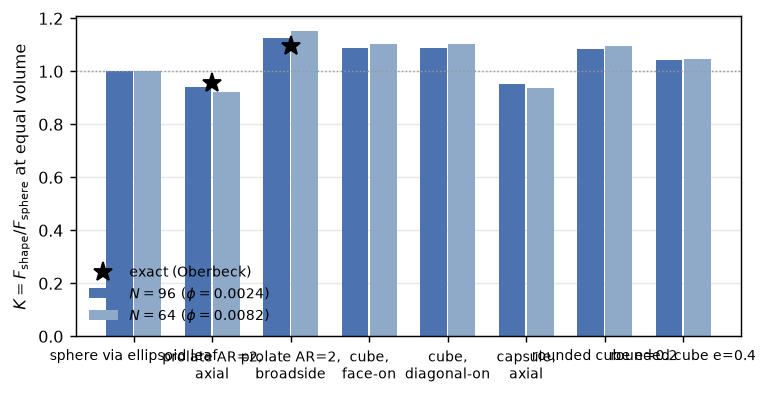

Figure 1: Equal-volume drag ratios in two box sizes. Filled markers are the exact Oberbeck values for the spheroid; the box shift is the honest uncertainty on every bar.

The cube, and what the correlations say about it

A cube has cubic symmetry, so its translational resistance tensor — a second-rank tensor invariant under that symmetry group — must be isotropic. Its Stokes drag is therefore independent of orientation, which is why we measure it twice, face-on and with a body diagonal along the flow. Any difference between those two is our discretisation error, measured directly.

Sphericity \(\psi = A_{\text{sphere of equal volume}} / A_{\text{particle}}\) compresses a shape to one number. Leith (1987) instead keeps two length scales — the projected-area-equivalent diameter \(d_n\) and the surface-equivalent diameter \(d_s\) — and predicts, in the Stokes regime,

\[ K_{\text{Leith}} = \tfrac{1}{3}\frac{d_n}{d_v} + \tfrac{2}{3}\frac{d_s}{d_v} . \tag{3}\]

Because \(d_n\) depends on orientation, Equation 3 does too: for a cube it runs 1.0457 face-on, 1.1031 edge-on and 1.1416 corner-on — a 9% spread across orientations where the true spread is exactly zero. (By Cauchy’s theorem the orientation-averaged projected diameter of a convex body equals its surface-equivalent diameter, so Leith’s random-orientation value is exactly \(\psi^{-1/2} = 1.1139\).) Any \(d_n\)-based correlation is therefore wrong for a cube in all but one orientation. The established orientation-averaged value is \(\chi = 1.08\) (Fuchs 1964; Pettyjohn and Christiansen 1948) — a two-digit tabulation from free-settling experiments, so ±0.01 at best, and not something to validate against to three digits.

One more consequence of the symmetry: a cube also has a centre of symmetry, so its translation–rotation coupling tensor vanishes and it settles without rotating. And all of this is a Stokes-flow statement: orientation dependence returns at finite Reynolds number.

Haider & Levenspiel is not a Stokes-regime reference

The most-cited non-spherical drag correlation (Haider and Levenspiel 1989) writes \(C_D = (24/\mathrm{Re})[1 + A\,\mathrm{Re}^{B}] + C/(1 + D/\mathrm{Re})\). Since \(B(\psi) = 0.0964 + 0.5565\psi > 0\) for every sphericity, \(A\,\mathrm{Re}^{B} \to 0\) and \(C\mathrm{Re}/D \to 0\) as \(\mathrm{Re}\to 0\): the correlation degenerates to \(C_D = 24/\mathrm{Re}\), the sphere, with no shape dependence at all. It cannot be compared against here, and that is a property of the correlation rather than a limitation of the measurement.

def geom_diameters(area_surface, area_projected):
    d_v = 2 * RV
    return d_v, np.sqrt(area_surface / np.pi), 2 * np.sqrt(area_projected / np.pi)

side = 2 * HC
cube_S, cube_A = 6 * side ** 2, side ** 2                       # face-on projection
d_v, d_s, d_n = geom_diameters(cube_S, cube_A)
K_leith_face = (1 / 3) * (d_n / d_v) + (2 / 3) * (d_s / d_v)
K_leith_rand = d_s / d_v                                        # Cauchy: <d_n> = d_s
psi_cube = (np.pi ** (1 / 3) * (6 * VOL) ** (2 / 3)) / cube_S
K_cube_face = lam["cube, face-on"] / lam["sphere (exact leaf)"]
K_cube_diag = lam["cube, diagonal-on"] / lam["sphere (exact leaf)"]
print("cube: side %.4f   S=%.2f   A_proj(face)=%.2f   d_s/d_v=%.4f  d_n/d_v=%.4f   sphericity %.4f"
      % (side, cube_S, cube_A, d_s / d_v, d_n / d_v, psi_cube))
print("   ISOTROPY CHECK (cubic symmetry says these are the same number):")
print("      face-on      K = %.5f" % K_cube_face)
print("      diagonal-on  K = %.5f      difference %+.3f%%"
      % (K_cube_diag, 100 * (K_cube_diag / K_cube_face - 1)))
print("   references:  orientation-averaged chi = 1.08 (Fuchs 1964 / Pettyjohn & Christiansen 1948,"
      " 2 digits)")
print("                Leith (1987) face-on %.4f    random-orientation %.4f"
      % (K_leith_face, K_leith_rand))
print("   measured (mean of the two orientations) = %.5f   -> %+.2f%% of the 1.08 datum"
      % (0.5 * (K_cube_face + K_cube_diag), 100 * (0.5 * (K_cube_face + K_cube_diag) / 1.08 - 1)))

cube: side 12.8959   S=997.83   A_proj(face)=166.31   d_s/d_v=1.1139  d_n/d_v=0.9095   sphericity 0.8060
   ISOTROPY CHECK (cubic symmetry says these are the same number):
      face-on      K = 1.08920
      diagonal-on  K = 1.08772      difference -0.136%
   references:  orientation-averaged chi = 1.08 (Fuchs 1964 / Pettyjohn & Christiansen 1948, 2 digits)
                Leith (1987) face-on 1.0457    random-orientation 1.1139
   measured (mean of the two orientations) = 1.08846   -> +0.78% of the 1.08 datum

Rounded cubes against a boundary-element model

Štrakl et al. (2022) published resistance tensors for superellipsoids in Stokes flow together with their code. Their shape family is the same as core’s, but written in the reciprocal convention: their blockiness \(e\) (with \(e=1\) a sphere and \(e\to 0\) a box) is \(n = 2/e\) in core’s exponent. Both are called “\(e\)” in their respective docs, which is exactly the kind of thing that silently produces a wrong comparison, so the code above states the mapping and checks it against the \(n=2\) sphere limit. Their model’s own error floor is about 0.05% (a sphere control returns \(\chi = 1.0005\)), and \(e = 0.2\) (\(n = 10\)) sits at the edge of their fitted range, so it is an extrapolation toward the sharp cube rather than a converged value.

STRAKL = {0.2: 1.0563, 0.4: 1.0255}      # chi = F_shape / F_equal-volume-sphere
print("   e     measured K (N=%d)    Strakl et al. (2022)    difference" % N_MAIN)
for e in (0.2, 0.4):
    k = lam["rounded cube e=%.1f" % e] / lam["sphere (exact leaf)"]
    print("   %.1f      %.5f              %.4f                 %+.2f%%"
          % (e, k, STRAKL[e], 100 * (k / STRAKL[e] - 1)))
print("   for scale: the sharp cube is %.5f (measured) against 1.08 (tabulated)"
      % (0.5 * (K_cube_face + K_cube_diag)))

   e     measured K (N=96)    Strakl et al. (2022)    difference
   0.2      1.08363              1.0563                 +2.59%
   0.4      1.04143              1.0255                 +1.55%
   for scale: the sharp cube is 1.08846 (measured) against 1.08 (tabulated)

The error budget

Two systematics survive the ratio, and both are measurable rather than estimated.

The box does not cancel exactly. The ratio method assumes an equal-volume shape and sphere block a periodic box equally. They do not: an elongated body blocks differently from a compact one, and the two boxes above disagree by 0.5–2.2% on exactly the shapes that are least sphere-like. That shift is the error bar.

The discrete body is not the analytic one — but by less than the obvious estimate. The solver’s own count of masked staggered points is a point sample of the shape, and a body with flat faces aligned to the grid samples badly at \(R_v = 8\) cells. The naive correction is that a volume mismatch \(\eta\) biases an equal-volume drag ratio by about \(\eta/3\). Both columns are below; read them together, because the naive correction turns out to be wrong.

print("   shape                          V_disc/V_an   implied drag bias   box shift (96->64)")
for k, k96, k64 in rows:
    eta = VSOL[(k, N_MAIN)] / VOL
    ref = VSOL[("sphere (exact leaf)", N_MAIN)] / VOL
    print("   %-28s   %+6.2f%%        %+6.2f%%             %+6.2f%%"
          % (k, 100 * (eta - 1), 100 * ((eta / ref) ** (1 / 3.0) - 1), 100 * (k64 / k96 - 1)))

   shape                          V_disc/V_an   implied drag bias   box shift (96->64)
   sphere via ellipsoid leaf       -1.90%         +0.00%              -0.00%
   prolate AR=2, axial             +0.44%         +0.79%              -1.82%
   prolate AR=2, broadside         -0.96%         +0.32%              +2.23%
   cube, face-on                   -5.44%         -1.22%              +1.17%
   cube, diagonal-on               -1.06%         +0.28%              +1.51%
   capsule, axial                  -2.18%         -0.10%              -1.62%
   rounded cube e=0.2              +5.47%         +2.44%              +1.03%
   rounded cube e=0.4              -0.87%         +0.35%              +0.49%

The point count is not the effective volume. The same cube, face-on and corner-on, samples 4.4 percentage points differently (−5.44% against −1.06%) — and its drag changes by 0.14%. The cut-cell geometry is built from surface crossings and apertures, not from counting masked points, and is correspondingly insensitive to that count; the \(\eta/3\) estimate is an upper bound that the solver comfortably beats. The one row where the two do track is the sharpest shape, the \(e = 0.2\) rounded cube: +5.5% in count and +2.6% above Štrakl’s value. That is the least trustworthy number on the page, and it is flagged rather than explained away.

So the residuals are the box. The spheroid’s exact gate misses by −1.6% and +2.9%, against a box shift of −1.8% and +2.2% in the same directions — an elongated body simply does not block a periodic cell the way an equal-volume sphere does, and the ratio does not cancel it. The method is sound and the numbers are box-limited rather than model-limited, which says what to do about it (a larger box, or a genuinely unbounded formulation) instead of declaring 3% a success.

Results

claim	measured	reference
sphere in the box (the calibration)	1.29739	Hasimoto/Sangani–Acrivos 1.30552 (-0.62%)
bound-leaf ellipsoid vs exact-distance sphere leaf, same shape	+0.000%	0
prolate AR=2, axial	0.94058	exact 0.95557 (-1.57%)
prolate AR=2, broadside	1.12615	exact 1.09443 (+2.90%)
spheroid anisotropy \(F_\perp/F_\parallel\)	1.19730	exact 1.14532
cube (face-on / diagonal-on)	1.08920 / 1.08772 (spread 0.136%, cubic symmetry says 0)	orientation-averaged \(\chi = 1.08\) (+0.78%); Leith face-on 1.0457
rounded cube \(e=0.2\)	1.08363	Štrakl et al. 1.0563 (+2.59%)
rounded cube \(e=0.4\)	1.04143	Štrakl et al. 1.0255 (+1.55%)
capsule, axial	0.95417	— (prediction)

The headline: a cube’s Stokes drag comes out orientation-independent to 0.14%, which cubic symmetry demands and no correlation built on projected area can reproduce — Leith’s own prediction for the same cube swings 9% between face-on and corner-on — and its value, 1.08846 against the tabulated \(\chi = 1.08 \pm 0.01\), sits inside the reference’s own uncertainty. The method that produced it was validated first against the exact Oberbeck spheroid, where it lands within the box error bar, and the sphere calibration reproduces the Hasimoto–Sangani–Acrivos periodic series to 0.62% with a fixed point independent of the time step to 3.7e-04.

One incidental result worth keeping: a sphere authored through the bound-only ellipsoid leaf and through the distance-exact sphere leaf give drag coefficients identical to six digits. The cut-cell geometry is derived from the zero level set and the crossings along grid lines, both of which a bound gets exactly right; the distance away from the surface, which is what the bound sacrifices, never enters. That is why the superquadric and ellipsoid measurements above are trustworthy at all.

Adapt this yourself

Any shape. Anything you can build in peclet.core.geom — a CSG difference, an instanced cluster — drops straight into SHAPES. Keep the volume fixed (body_properties will tell you what it is) and the ratio stays meaningful.
Orientation sweeps. Rotate the instance quaternion rather than re-authoring the leaf, and the drag becomes a function of angle: the anisotropy the correlations cannot express.
Finite Reynolds number. set_advection(True) — the reaction budget carries explicit advection, so the same force call remains valid, and the correlations start earning their keep.
Feed it to DEM. The same tree is a peclet.dem particle via scene_particle.build; the measured \(K\) is the drag closure a point-particle CFD-DEM run would need.

Reproduce this

PECLET_LOCAL_BUILD=/path/to/suite/flow/build_l3_cuda \
  quarto render examples/nonsphere-drag/index.qmd --execute

References

Fuchs, N. A. 1964. The Mechanics of Aerosols. Pergamon Press.

Haider, A., and O. Levenspiel. 1989. “Drag Coefficient and Terminal Velocity of Spherical and Nonspherical Particles.” Powder Technology 58 (1): 63–70. https://doi.org/10.1016/0032-5910(89)80008-7.

Leith, David. 1987. “Drag on Nonspherical Objects.” Aerosol Science and Technology 6 (2): 153–61. https://doi.org/10.1080/02786828708959128.

Pettyjohn, E. S., and E. B. Christiansen. 1948. “Effect of Particle Shape on Free-Settling Rates of Isometric Particles.” Chemical Engineering Progress 44 (2): 157–72.

Štrakl, Mitja, Matjaž Hriberšek, Jana Wedel, Paul Steinmann, and Jure Ravnik. 2022. “A Model for Translation and Rotation Resistance Tensors for Superellipsoidal Particles in Stokes Flow.” Journal of Marine Science and Engineering 10 (3): 369. https://doi.org/10.3390/jmse10030369.