import importlib.util, os, subprocess, sys
_local = os.environ.get("PECLET_LOCAL_BUILD")
if _local:
    for p in _local.split(os.pathsep):
        sys.path.insert(0, p)
elif importlib.util.find_spec("peclet") is None:
subprocess.run([sys.executable, "-m", "pip", "install", "-q", "peclet"], check=True)Backward-facing step: separated flow and reattachment
A stream expands over a step, separates, and reattaches downstream — the canonical benchmark for separated internal flow, with the step realized purely as an inlet profile.
flow
inflow-outflow
boundary-conditions
separation
verification
 Runs on a free Colab CPU runtime — the first cell installs
 peclet from PyPI.
What you’ll learn
The backward-facing step (BFS) is the textbook benchmark for separated internal flow. A channel flow expands abruptly over a step; the stream cannot turn the corner, so it separates at the step edge, encloses a slow recirculation bubble on the wall behind the step, and reattaches further downstream. The reattachment length \(x_r\) grows with Reynolds number — a quantity measured in countless experiments (Armaly et al. 1983) and computations (Gartling 1990).
Two things make this a nice peclet.flow example:
- The step is an inlet condition, not geometry. Instead of meshing a step, we feed the developed upper-half parabola into the inlet and prescribe zero over the lower half (the step face) with
set_domain_bc_profile. The expansion, separation and bubble then emerge from the flow. - It exercises the full inflow/outflow machinery — a per-position velocity inlet, a zero-gradient outflow, and the projection that lets mass leave — on a genuinely separated flow with reverse velocity near the wall.
Setup
Gartling’s expansion-ratio-2 geometry: full height \(H = 2S\) (\(S\) = step height), length \(L = 12S\), no-slip walls top and bottom. The inlet (\(-x\)) carries the developed parabola over the open upper half \(y \in [S, 2S]\) and zero over the step face \(y \in [0, S]\); the outlet (\(+x\)) is zero-gradient. The step Reynolds number is \(\mathrm{Re}_S = U_{in} S/\nu\) with \(U_{in}\) the mean inlet velocity over the open half.
A note on the time step: the shear layer springing off the step lip is stiff for the explicit high-order (SOU) advection correction, so we march at dt=0.2 — comfortably under its stability limit while keeping full second-order accuracy. (Larger steps show a roundoff-sensitive transient that can diverge; set_deferred_correction(False) — pure first-order upwind — is the cheap robust alternative.)
import numpy as np
import matplotlib.pyplot as plt
from peclet import flow

plt.rcParams.update({"figure.dpi": 130, "font.size": 10, "axes.grid": True,
                     "grid.alpha": 0.3, "axes.axisbelow": True,
                     "figure.facecolor": "white", "savefig.bbox": "tight"})
BLUE, RED = "#1f77b4", "#d62728"
The solve
The whole simulation is the function below — the step lives entirely in the inlet profile (parabola over the open half, zero over the step face):
def inlet_profile(H, S, nz, U):
    """Developed parabola over the open upper half [S, 2S], zero over the step face [0, S]."""
    prof = np.zeros((H, nz, 3))
    yc = np.arange(H) + 0.5
    eta = (yc - S) / S
    prof[yc > S, :, 0] = (6.0 * U * eta * (1 - eta))[yc > S, None]
    return prof

def reattachment(u_bottom):
    """End of the bubble: first reverse -> forward crossing of the near-wall streamwise velocity."""
    rev = False
    for i in range(1, len(u_bottom)):
        if u_bottom[i] < 0.0:
            rev = True
        elif rev and u_bottom[i] >= 0.0:
            return (i - 1) + u_bottom[i - 1] / (u_bottom[i - 1] - u_bottom[i])
    return 0.0

def solve_bfs(Re, S=16, Lr=12, U=1.0, nz=4, dt=0.2, steps=12000):
    H, L = 2 * S, Lr * S
    nu = U * S / Re
    s = flow.Solver(L, H, nz)
    s.set_rho(1.0); s.set_mu(nu); s.set_dt(dt); s.set_advection(True)
    s.set_domain_bc_profile(0, inlet_profile(H, S, nz, U))   # inlet == the step
    s.set_domain_bc(1, 3)                                     # outflow
    s.set_domain_bc(2, 1); s.set_domain_bc(3, 1)             # no-slip walls
    s.set_velocity_solver_params(60)
    s.set_pressure_multigrid(True, levels=8)
    s.set_pressure_solver_params(80)
    s.set_pressure_geometry(np.full((L, H, nz), 1e30, order="F"))
    for _ in range(steps):
        s.step()
    u = s.get_u()[:, :, nz // 2]; v = s.get_v()[:, :, nz // 2]
    return dict(u=u, v=v, xr_S=reattachment(u[:, 0]) / S, S=S, H=H, L=L, Re=Re)
Each Reynolds number marches ~12000 steps to steady state (about half an hour on a GPU build, a couple of hours on CPU), so the two solutions are cached in bfs_cache.npz and the page loads them. Delete that file — or run make_cache.py on a GPU build — to recompute from scratch.
import os, urllib.request
CACHE = "bfs_cache.npz"
if not os.path.exists(CACHE):
    url = ("https://raw.githubusercontent.com/computational-chemical-engineering/"
           "peclet-examples/main/examples/backward-facing-step/bfs_cache.npz")
    try:
        urllib.request.urlretrieve(url, CACHE)
    except Exception:
        pass
if os.path.exists(CACHE):
    _d = np.load(CACHE)
    cache = {k: (_d[k].item() if _d[k].ndim == 0 else _d[k]) for k in _d.files}
    runs = {Re: {"u": cache[f"u_{Re}"], "v": cache[f"v_{Re}"], "xr_S": float(cache[f"xr_S_{Re}"]),
                 "H": int(cache["H"]), "L": int(cache["L"]), "S": int(cache["S"])}
            for Re in (100, 200)}
    print(f"loaded cached result — grid {cache['L']}x{cache['H']}  "
          f"(delete {CACHE} to recompute)")
else:
    runs = {int(r["Re"]): r for r in (solve_bfs(100.0), solve_bfs(200.0))}
    print("computed from scratch")
S = runs[100]["S"]
loaded cached result — grid 192x32 (delete bfs_cache.npz to recompute)The recirculation bubble
Streamlines make the separation visible: the incoming jet rides over the top, a slow clockwise recirculation bubble fills the corner behind the step, and the flow reattaches to the bottom wall at \(x_r\) (marked). Raising the Reynolds number stretches the bubble downstream.
fig, axes = plt.subplots(2, 1, figsize=(9, 4.4), sharex=True)
for ax, Re in zip(axes, (100, 200)):
    r = runs[Re]
    L, H = r["L"], r["H"]
    x = np.arange(L) + 0.5; y = np.arange(H) + 0.5
    X, Y = np.meshgrid(x, y)
    speed = np.sqrt(r["u"] ** 2 + r["v"] ** 2)
    ax.streamplot(x, y, r["u"].T, r["v"].T, density=1.4, linewidth=0.6,
                  color=speed.T, cmap="viridis", arrowsize=0.6)
    ax.axhline(S, xmax=0.02, color="k", lw=3)                 # the step face at the inlet
    ax.plot(r["xr_S"] * S, 0.7, marker="v", color=RED, ms=9, clip_on=False)
    ax.set(ylim=(0, H), ylabel="y",
           title=f"Re_S = {Re}   —   reattachment  x_r/S = {r['xr_S']:.1f}")
    ax.grid(False)
axes[-1].set_xlabel("x")
plt.show()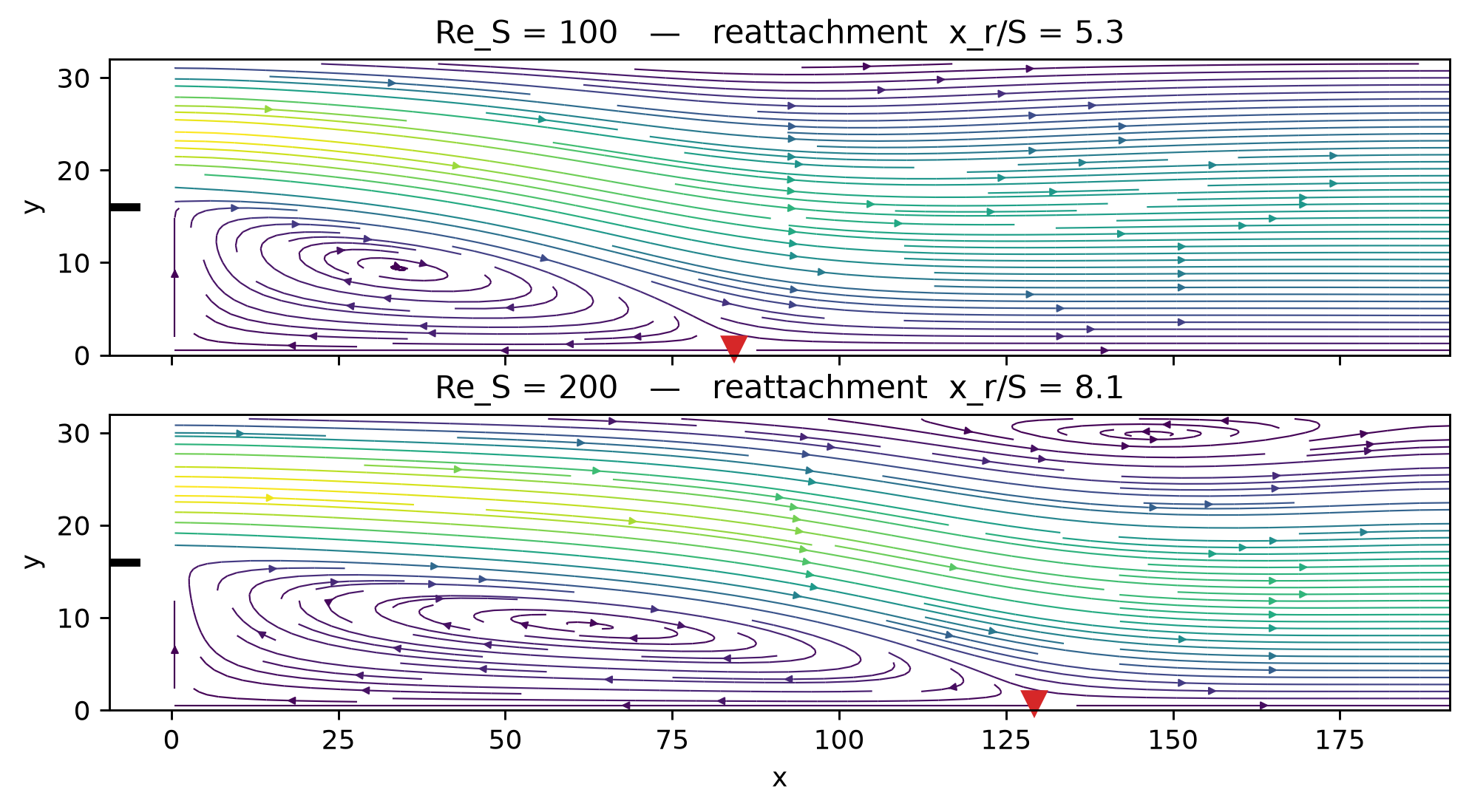
Reattachment length vs Reynolds number
In the laminar regime the reattachment length grows roughly linearly with \(\mathrm{Re}_S\). Our two points sit on the Armaly/Biswas trend — the standard quantitative check for a BFS solver.
Re_pts = np.array([100, 200])
xr_pts = np.array([runs[100]["xr_S"], runs[200]["xr_S"]])
fig, ax = plt.subplots(figsize=(5.2, 3.8))
# reference laminar band (Armaly/Biswas): x_r/S ~ 5 at Re_S=100, ~8 at Re_S=200
ax.fill_between([80, 220], [4.2, 7.0], [5.8, 9.4], color=BLUE, alpha=0.12,
                label="laminar reference band")
ax.plot(Re_pts, xr_pts, "o-", color=RED, ms=9, label="peclet.flow")
for Re, xr in zip(Re_pts, xr_pts):
    ax.annotate(f"{xr:.1f}", (Re, xr), textcoords="offset points", xytext=(8, -4), fontsize=9)
ax.set(xlabel="Re_S = U_in S / nu", ylabel="reattachment  x_r / S",
       title="Reattachment grows with Reynolds number", xlim=(80, 220))
ax.legend(fontsize=8)
plt.show()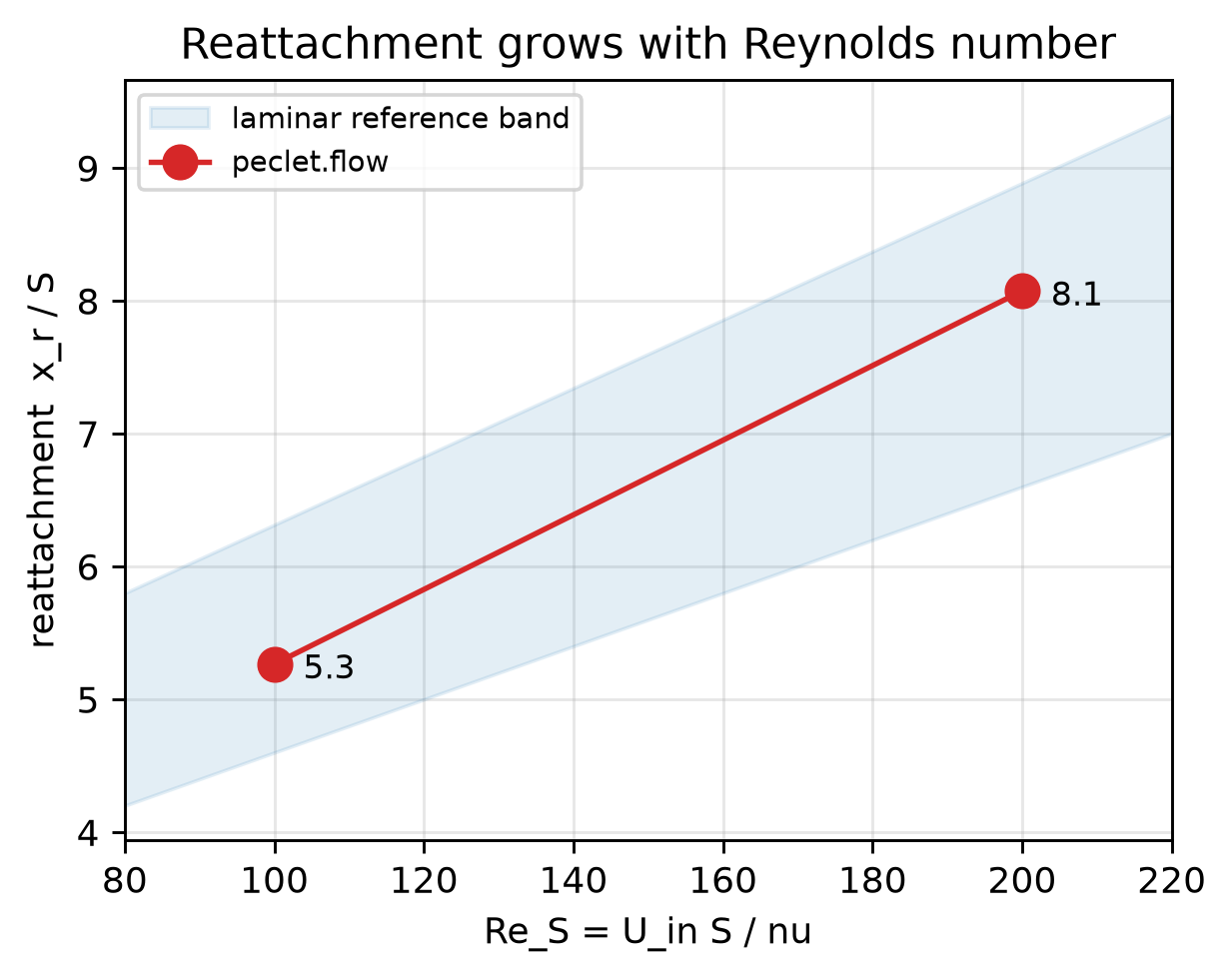
Takeaways
- The step is realized as an inlet profile — no immersed geometry — and the separation, recirculation bubble and reattachment emerge from the flow.
- The reattachment length grows with \(\mathrm{Re}_S\), tracking the laminar Armaly/Biswas benchmark — a genuine quantitative validation of the inflow/outflow solver on a separated flow.
- Separated shear layers are numerically stiff for explicit advection corrections; a modest time step (or first-order upwind via
set_deferred_correction(False)) keeps the march robust.
Reproduce this
# From PyPI (CPU; the two solves take a couple of hours):
pip install peclet
python examples/backward-facing-step/make_cache.py   # writes bfs_cache.npz, then: quarto render

# From a local build (GPU ~2x faster — the RTX-class card does each Re in ~30 min):
PECLET_LOCAL_BUILD=/path/to/suite/flow/build_cuda \
  python examples/backward-facing-step/make_cache.py
quarto render examples/backward-facing-step/index.qmd --execute
References: B. F. Armaly, F. Durst, J. C. F. Pereira, B. Schönung, Experimental and theoretical investigation of backward-facing step flow, J. Fluid Mech. 127 (1983) 473–496. — D. K. Gartling, A test problem for outflow boundary conditions, Int. J. Numer. Methods Fluids 11 (1990) 953–967.