import importlib.util, os, subprocess, sys
_local = os.environ.get("PECLET_LOCAL_BUILD")
if _local:
    for p in _local.split(os.pathsep):
        sys.path.insert(0, p)
elif importlib.util.find_spec("peclet") is None:
subprocess.run([sys.executable, "-m", "pip", "install", "-q", "peclet"], check=True)Oscillating sphere: unsteady Stokes drag vs Stokes (1851)
A sphere that never moves, only its boundary condition — the linearised limit where the exact complex drag has an in-phase and an out-of-phase part, and a periodic box that screens its own images.
flow
IBM
moving-geometry
verification
analytic
GPU
 GPU example — the frozen page reads correctly without a solver; re-executing wants a CUDA build.
What you’ll learn
Stokes solved the oscillating sphere in 1851 and the answer is complex: the drag has a part in phase with the velocity (enhanced viscous drag) and a part in phase with the acceleration (added mass plus flow history). Reproducing both is a much stronger test of an unsteady incompressible solver than any steady drag, because the two parts fail differently — a wrong time term shows up in the imaginary part alone.
This page uses it to exercise three things at once:
peclet.flow’s moving-geometry path — the boundary condition on a cut cell becomes the local wall velocity instead of zero.- The discrete-reaction hydrodynamic force (
hydro_force_torque_reaction), which takes the force from the momentum the fluid actually lost rather than from a reconstructed surface traction. In an unsteady problem that distinction is the whole game: the time term is part of the budget by construction. - What a periodic box does to an unsteady problem — and it is not what it does to a steady one. That turns out to be the most interesting result on the page, and it is measured, not asserted.
The physics
A sphere of radius \(R\) oscillating with velocity \(U(t) = \operatorname{Re}[\hat U e^{-i\omega t}]\) in an unbounded incompressible fluid feels
\[ \hat F = -6\pi\mu R\,\hat U \left[\,1 + \lambda R + \tfrac{1}{9}(\lambda R)^2\right], \qquad \lambda^2 = -\frac{i\omega}{\nu},\ \ \operatorname{Re}\lambda > 0 , \tag{1}\]
so with \(\delta = \sqrt{2\nu/\omega}\) the Stokes layer thickness, \(\lambda R = (1-i)R/\delta\). The bracket is the complex drag coefficient \(C\); \(\operatorname{Re} C = 1 + R/\delta\) is the in-phase (dissipative) part, growing above the steady value 1 as the layer thins, and \(\operatorname{Im} C = -R/\delta - \tfrac{2}{9}(R/\delta)^2\) is the out-of-phase (added-mass and history) part. (Stokes 1851; Landau & Lifshitz, Fluid Mechanics §24, problem 5.)
The implementation insight. Equation 1 is the solution of the linearised problem, in which the amplitude \(A/R \to 0\) and the no-slip condition is applied at the sphere’s mean position. The geometry therefore never moves: we install a static sphere and give it a sinusoidal wall velocity. No fresh cells, no moving interface, and — rigorously in this limit — no advection.
Setup
NoteRequires a recent
peclet
The analytic-scene API (set_scene, set_instance_motion, rebuild_geometry) and the discrete-reaction force (hydro_force_torque_reaction) are newer than the current PyPI release. The page is frozen, so it renders correctly regardless; re-executing it needs a source build.
import time
import numpy as np
import matplotlib.pyplot as plt
from peclet import flow as sdflow

plt.rcParams.update({"figure.dpi": 130, "font.size": 9, "axes.axisbelow": True,
                     "figure.facecolor": "white", "savefig.bbox": "tight"})

RHO, MU = 1.0, 0.1          # everything in cell units: h = 1, so lengths are in cells
NU = MU / RHO
U0 = 0.02                   # wall-velocity amplitude
KN_R, KI_I, KI_R = 16, 2, 17   # scene encoding strides
Kokkos::OpenMP::initialize WARNING: OMP_PROC_BIND environment variable not set
In general, for best performance with OpenMP 4.0 or better set OMP_PROC_BIND=spread and OMP_PLACES=threads
For best performance with OpenMP 3.1 set OMP_PROC_BIND=true
For unit testing set OMP_PROC_BIND=false
The scene is one sphere instance in a periodic box. set_scene takes the flat node/instance encoding; set_solid_from_scene derives the cut-cell geometry from it analytically — no sampled SDF, no lattice.
def solver(n, r, dt, u_init):
    node_ints = np.array([1, -1, -1], dtype=np.int32)          # one kSphere leaf
    node_reals = np.zeros(KN_R); node_reals[0] = r
    node_reals[14] = 1.0; node_reals[15] = 1.0                 # identity transform: quat w, scale
    inst_ints = np.zeros((1, KI_I), dtype=np.int32); inst_ints[0] = (0, -1)
    inst_reals = np.zeros((1, KI_R))
    inst_reals[0, 0:3] = (0.5 * n,) * 3                        # centred
    inst_reals[0, 6] = 1.0; inst_reals[0, 7] = 1.0

    s = sdflow.Solver(n, n, n)
    s.set_rho(RHO); s.set_mu(MU); s.set_dt(dt)
    s.set_advection(False)                                     # exact in the linearised limit
    s.set_velocity_solver_params(100)
    s.set_pressure_solver_params(25)
    s.set_pressure_multigrid(True, levels=4)                   # depth >= 4: levels=1 is a 50x tax
    s.set_scene(node_ints, node_reals, inst_ints.ravel(), inst_reals.ravel(), periodic=True)
    s.set_instance_motion(0, lin_vel=[u_init, 0.0, 0.0])
    s.set_solid_from_scene(True)
    return s
Step 1 — Calibrate the box against Hasimoto
Before any unsteady claim, check the steady one. A single sphere in a periodic box is a simple-cubic array, whose Stokes drag ratio Hasimoto (1959) gives as a series in the solid fraction \(c\), extended by Sangani & Acrivos (1982):
\[ K = \Big[\,1 - 1.7601\,c^{1/3} + c - 1.5593\,c^{2} + 3.9799\,c^{8/3} - 3.0734\,c^{10/3}\,\Big]^{-1}. \tag{2}\]
The last two terms are not decoration: at \(c = 0.125\) the four-term series gives 4.533 and this one gives 4.289, against Zick & Homsy’s tabulated 4.292. This is a check of the geometry, the cut-cell operator and the reaction force at once, against a result that owes nothing to our discretisation.
One convention has to be nailed down. The drag ratio depends on which mean velocity normalises it — superficial (volume-averaged over the whole cell, sphere interior included) or interstitial (over the fluid only) — and the two differ by a factor \((1-c)\). We use the superficial one, and the data say that is right: fitting \(1/K = 1 + A c^{1/3} + B c\) through the three dilutions below recovers \(B = 0.90\) under the superficial convention against the series’ exact 1, and \(B = 1.34\) under the interstitial one.
_SCACHE = {}

def steady_lambda(n, r, f=1e-4, dt=200.0, tol=1e-7, maxit=4000):
    key = (n, round(r, 6), f, dt, tol, maxit)
    if key not in _SCACHE:
        _SCACHE[key] = _steady_lambda(n, r, f, dt, tol, maxit)
    return _SCACHE[key]

def _steady_lambda(n, r, f, dt, tol, maxit):
    """Fixed sphere, uniform body force; iterate to a genuinely steady mean velocity."""
    s = solver(n, r, dt, 0.0)
    s.set_body_force(f, 0.0, 0.0)
    nc = s.fluid_momentum_cells()[0]
    prev, it = 0.0, 0
    while it < maxit:
        s.step(); it += 1
        um = float(np.asarray(s.get_u()).sum()) / nc
        if it > 5 and abs(um - prev) < tol * abs(um):
            break
        prev = um
    force = float(np.asarray(s.hydro_force_torque_reaction())[0][0][0])
    return force / (6 * np.pi * MU * r * um), um, it

def hasimoto(c):
    """Hasimoto (1959) extended by Sangani & Acrivos (1982), simple-cubic array."""
    return 1.0 / (1 - 1.7601 * c ** (1 / 3) + c - 1.5593 * c ** 2
                  + 3.9799 * c ** (8 / 3) - 3.0734 * c ** (10 / 3))

print("(a) GRID ladder at FIXED c: is the steady drag converged?")
steady_rows = []
for n, r in ((64, 9.60), (96, 14.40)):
    c = (4 / 3) * np.pi * r ** 3 / n ** 3
    lam_i, um, it = steady_lambda(n, r)           # interstitial normalisation
    lam_s = lam_i / (1 - c)                       # superficial
    steady_rows.append((n, r, c, lam_i, lam_s, hasimoto(c), it))
    print("    N=%3d  R=%5.2f h  c=%.5f   lambda=%.5f (superficial)   series=%.5f   %+.2f%%   "
          "(%d steps)" % (n, r, c, lam_s, hasimoto(c), 100 * (lam_s / hasimoto(c) - 1), it))

print("(b) DILUTION ladder at FIXED R = 9.6 h: where do the conventions stop mattering?")
dil_rows = []
for n in (64, 96, 128):
    r = 9.60
    c = (4 / 3) * np.pi * r ** 3 / n ** 3
    lam_i, um, it = steady_lambda(n, r)
    lam_s = lam_i / (1 - c)
    dil_rows.append((n, c, lam_i, lam_s, hasimoto(c)))
    print("    c=%.5f   superficial %.5f (%+.2f%%)   interstitial %.5f (%+.2f%%)   series %.5f"
          % (c, lam_s, 100 * (lam_s / hasimoto(c) - 1), lam_i,
             100 * (lam_i / hasimoto(c) - 1), hasimoto(c)))

# which convention reproduces the series' own O(c) coefficient?
def fit_AB(vals):
    cs = np.array([r[1] for r in dil_rows]); y = np.array(vals) - 1.0
    M = np.column_stack([cs ** (1 / 3), cs])
    return np.linalg.lstsq(M, y, rcond=None)[0]
A_s, B_s = fit_AB([1 / r[3] for r in dil_rows])
A_i, B_i = fit_AB([1 / r[2] for r in dil_rows])
print("    series coefficients 1/K = 1 + A c^(1/3) + B c:   exact A=-1.7601  B=+1.0000")
print("       superficial  A=%+.4f  B=%+.4f          interstitial  A=%+.4f  B=%+.4f"
      % (A_s, B_s, A_i, B_i))
(a) GRID ladder at FIXED c: is the steady drag converged?
N= 64 R= 9.60 h c=0.01414 lambda=1.67437 (superficial) series=1.69987 -1.50% (671 steps)
N= 96 R=14.40 h c=0.01414 lambda=1.67562 (superficial) series=1.69987 -1.43% (1430 steps)
(b) DILUTION ladder at FIXED R = 9.6 h: where do the conventions stop mattering?
c=0.01414 superficial 1.67437 (-1.50%) interstitial 1.65070 (-2.89%) series 1.69987
c=0.00419 superficial 1.38151 (-0.47%) interstitial 1.37572 (-0.89%) series 1.38805
c=0.00177 superficial 1.26559 (-0.15%) interstitial 1.26336 (-0.33%) series 1.26748
series coefficients 1/K = 1 + A c^(1/3) + B c: exact A=-1.7601 B=+1.0000
superficial A=-1.7553 B=+1.5374 interstitial A=-1.7507 B=+2.0657Step 2 — Oscillate the wall
set_instance_motion sets the instance’s rigid-body velocity, but it does not on its own reach the fields that carry it into the solve: the momentum operator’s no-slip datum and the cut-cell projection’s wall flux are both built where the geometry is, in set_solid_from_scene. A time-varying wall velocity therefore needs one call per step to rebuild them.
refresh_wall_velocity() is that call. It re-derives the wall-velocity fields and the momentum stencils and nothing else, and it refuses if an instance transform has changed since the last geometry build — because it does not re-sample the SDF, the apertures or the pressure operator, and on a body that had actually moved it would silently continue on stale geometry. For this page the transforms never change, which is exactly its scope.
The alternative is rebuild_geometry(), which re-derives everything and gives bitwise-identical fields here; it costs 4.0 ms against 1.4 ms at \(N=48\) on this GPU, against a bare step of 12.4 ms. That is a 2.8× cheaper call and about 16% off the driver’s per-step total — worth having, and worth stating both ways rather than quoting only the 2.8×.
_CACHE = {}   # the ladders below deliberately overlap; each configuration is solved once

def oscillate(n, r, delta, spp=200, nper=4, fitp=2):
    key = (n, r, round(delta, 9), spp, nper, fitp)
    if key not in _CACHE:
        _CACHE[key] = _oscillate(n, r, delta, spp, nper, fitp)
    return _CACHE[key]

def _oscillate(n, r, delta, spp, nper, fitp):
    """Return the complex drag coefficient C = -F_hat / (6 pi mu R U_hat)."""
    om = 2 * NU / delta ** 2
    period = 2 * np.pi / om
    dt = period / spp
    s = solver(n, r, dt, U0)
    nc = s.fluid_momentum_cells()[0]
    t, force, umean = [], [], []
    t0 = time.time()
    for it in range(spp * nper):
        # The momentum solve is BACKWARD EULER, so its wall boundary condition belongs at the END
        # of the step. Imposing U(t^n) instead and labelling the result t^{n+1} rotates the fitted
        # phase by a full omega*dt -- 1.8 degrees at 200 steps per cycle -- which lands almost
        # entirely in the imaginary part. That is a bookkeeping error, not a solver one, and it is
        # larger than everything else on this page.
        now = (it + 1) * dt
        s.set_instance_motion(0, lin_vel=[U0 * np.cos(om * now), 0.0, 0.0])
        s.refresh_wall_velocity()               # the geometry is static; only the BC moves
        s.step()
        force.append(float(np.asarray(s.hydro_force_torque_reaction())[0][0][0]))
        t.append(now)
        umean.append(float(np.asarray(s.get_u()).sum()) / nc)
    t = np.array(t); force = np.array(force); umean = np.array(umean)
    keep = t >= (nper - fitp) * period                      # fit only the settled cycles
    basis = np.column_stack([np.cos(om * t[keep]), np.sin(om * t[keep])])
    cf, *_ = np.linalg.lstsq(basis, force[keep], rcond=None)
    cu, *_ = np.linalg.lstsq(basis, umean[keep], rcond=None)
    resid = np.linalg.norm(force[keep] - basis @ cf) / np.linalg.norm(force[keep])
    return (-(cf[0] + 1j * cf[1]) / (6 * np.pi * MU * r * U0),
            (cu[0] + 1j * cu[1]) / U0, resid, time.time() - t0,
            (t, force, om, period, basis, cf, keep))

def C_theory(delta, r):
    lr = (1 - 1j) / delta * r
    return 1 + lr + lr ** 2 / 9
N_SWEEP, R_SWEEP = 96, 9.6 # delta >= 4h needs delta/R >= 0.42 here
DRS = [0.5, 0.75, 1.0, 1.5, 2.5]
sweep, trace1 = [], None
for dr in DRS:
d = dr * R_SWEEP
C, uh, resid, wall, trace = oscillate(N_SWEEP, R_SWEEP, d)
Ct = C_theory(d, R_SWEEP)
sweep.append((dr, d, C, Ct, uh, resid, wall))
if dr == 1.0:
trace1 = trace
print("delta/R=%.2f delta=%5.2f h C = %+.5f %+.5fi Stokes = %+.5f %+.5fi"
" |dC|/|C| = %5.2f%% fit resid %.0e %3.0f s"
% (dr, d, C.real, C.imag, Ct.real, Ct.imag, 100 * abs(C - Ct) / abs(Ct), resid, wall))delta/R=0.50 delta= 4.80 h C = +3.00485 -2.87969i Stokes = +3.00000 -2.88889i |dC|/|C| = 0.25% fit resid 4e-04 88 s
delta/R=0.75 delta= 7.20 h C = +2.32851 -1.72144i Stokes = +2.33333 -1.72840i |dC|/|C| = 0.29% fit resid 4e-04 91 s
delta/R=1.00 delta= 9.60 h C = +1.99034 -1.21974i Stokes = +2.00000 -1.22222i |dC|/|C| = 0.43% fit resid 3e-04 84 s
delta/R=1.50 delta=14.40 h C = +1.64966 -0.76948i Stokes = +1.66667 -0.76543i |dC|/|C| = 0.95% fit resid 8e-04 84 s
delta/R=2.50 delta=24.00 h C = +1.36570 -0.44773i Stokes = +1.40000 -0.43556i |dC|/|C| = 2.48% fit resid 2e-03 84 sCode
dd = np.linspace(0.35, 3.0, 300)
Cth = np.array([C_theory(x * R_SWEEP, R_SWEEP) for x in dd])
fig, ax = plt.subplots(figsize=(6.0, 3.4))
ax.plot(dd, Cth.real, color="#4c72b0", lw=1.2, label=r"Stokes 1851: $\mathrm{Re}\,C$")
ax.plot(dd, Cth.imag, color="#c44e52", lw=1.2, label=r"Stokes 1851: $\mathrm{Im}\,C$")
ax.plot([s[0] for s in sweep], [s[2].real for s in sweep], "o", color="#4c72b0", ms=6,
        label="peclet.flow")
ax.plot([s[0] for s in sweep], [s[2].imag for s in sweep], "s", color="#c44e52", ms=6)
ax.axhline(1.0, color="0.7", lw=0.7, ls=":")
ax.set_xlabel(r"$\delta/R$"); ax.set_ylabel(r"$C = \hat F\,/\,(-6\pi\mu R\hat U)$")
ax.legend(fontsize=8, frameon=False); ax.grid(alpha=0.3)
plt.show()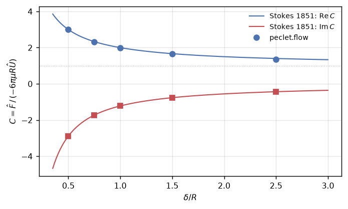
Code
t, force, om, period, basis, cf, keep = trace1
fig, ax = plt.subplots(figsize=(6.0, 2.6))
ax.plot(t / period, force, color="0.6", lw=0.9, label="measured $F_x(t)$")
ax.plot(t[keep] / period, basis @ cf, color="#c44e52", lw=1.3, ls="--", label="fitted harmonic")
ax.set_xlabel("cycles"); ax.set_ylabel("$F_x$")
ax.legend(fontsize=8, frameon=False); ax.grid(alpha=0.3)
plt.show()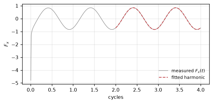
Step 3 — Where the residual comes from
ImportantThe largest error on this page was a bookkeeping one
The momentum solve is backward Euler, so its wall boundary condition belongs at \(t^{n+1}\). Imposing \(U(t^n)\) and labelling the resulting force \(t^{n+1}\) — the obvious loop to write — rotates the fitted phase by a full \(\omega\Delta t\), which is 1.8° at 200 steps per cycle and lands almost entirely in the imaginary part. Before the fix, \(\operatorname{Im} C\) sat at −1.155 against −1.222 and, worse, did not improve when the box grew, which looked like a modelling error. It was not. Both versions are one line apart; the correct one is in the driver above.
What is left has two systematic sources, and they separate cleanly because one is controlled by the time step and the other by the box:
| source | size | how it scales |
|---|---|---|
| time discretisation (backward Euler) | \(\mathcal{O}(\omega\Delta t)\) | shrinks with the time step |
| screened viscous images | \(\sim e^{-L/\delta}\) | negligible once \(\delta \ll L\) |
| potential (added-mass) images | \(\sim (R/L)^3\) | shrinks when the box grows |
| the unscreened \(k=0\) momentum mode | \(\mathcal{O}(c)\) | shrinks when the box grows |
Ct1 = C_theory(9.6, 9.6)
print("TIME-STEP ladder at N=64, delta/R = 1 (backward Euler -> first order in omega*dt)")
dt_rows = []
for spp in (100, 200, 400):
    C, _, _, wall, _ = oscillate(64, 9.6, 9.6, spp=spp)
    dt_rows.append((spp, C))
    print("    %4d steps/cycle   C = %+.5f %+.5fi   err %5.2f%%   (%3.0f s)"
          % (spp, C.real, C.imag, 100 * abs(C - Ct1) / abs(Ct1), wall))
rich = 2 * dt_rows[-1][1] - dt_rows[-2][1]          # first-order Richardson
print("    Richardson (dt -> 0)  C = %+.5f %+.5fi   err %5.2f%%"
      % (rich.real, rich.imag, 100 * abs(rich - Ct1) / abs(Ct1)))
TIME-STEP ladder at N=64, delta/R = 1 (backward Euler -> first order in omega*dt)
100 steps/cycle C = +1.95817 -1.20864i err 1.88% ( 23 s)
200 steps/cycle C = +1.94185 -1.21985i err 2.48% ( 46 s)
400 steps/cycle C = +1.93468 -1.22471i err 2.79% ( 75 s)
Richardson (dt -> 0) C = +1.92752 -1.22957i err 3.11%print("BOX ladder: L up at FIXED R = 9.6 h, delta/R = 1 and steps-per-cycle")
box_rows = []
for n in (64, 96, 128):
c = (4 / 3) * np.pi * 9.6 ** 3 / n ** 3
C, uh, resid, wall, _ = oscillate(n, 9.6, 9.6)
box_rows.append((n, c, C, abs(uh)))
print(" L/R=%5.2f c=%.2e C = %+.5f %+.5fi err %5.2f%% |<u>|/U0=%.4f "
"e^{-L/delta}=%.1e (%3.0f s)"
% (n / 9.6, c, C.real, C.imag, 100 * abs(C - Ct1) / abs(Ct1), abs(uh),
np.exp(-n / 9.6), wall))BOX ladder: L up at FIXED R = 9.6 h, delta/R = 1 and steps-per-cycle
L/R= 6.67 c=1.41e-02 C = +1.94185 -1.21985i err 2.48% |<u>|/U0=0.0739 e^{-L/delta}=1.3e-03 ( 46 s)
L/R=10.00 c=4.19e-03 C = +1.99034 -1.21974i err 0.43% |<u>|/U0=0.0221 e^{-L/delta}=4.5e-05 ( 84 s)
L/R=13.33 c=1.77e-03 C = +2.00245 -1.21741i err 0.23% |<u>|/U0=0.0093 e^{-L/delta}=1.6e-06 (134 s)The three terms that shrink when the box grows are the screened viscous images \(e^{-L/\delta}\) (already \(10^{-6}\) at the largest box — the oscillatory Stokeslet screens itself), the potential-part images \((R/L)^3\), and the unscreened \(k=0\) momentum mode, which is \(\mathcal{O}(c)\) and is the one still doing the work here.
Code
fig, (a1, a2) = plt.subplots(1, 2, figsize=(7.2, 2.9))
cs = np.array([b[1] for b in box_rows])
errs = np.array([100 * abs(b[2] - Ct1) / abs(Ct1) for b in box_rows])
a1.loglog(cs, errs, "o-", color="#c44e52")
a1.set_xlabel(r"solid fraction $c$ (box ladder)"); a1.set_ylabel("error in $C$ [%]")
a1.grid(which="both", alpha=0.3); a1.set_title("box ladder, $\\delta/R = 1$", fontsize=9)
sp = np.array([r[0] for r in dt_rows]); de = np.array([100 * abs(r[1] - Ct1) / abs(Ct1)
                                                       for r in dt_rows])
a2.loglog(1.0 / sp, de, "o-", color="#4c72b0", label="measured")
a2.loglog(1.0 / sp, de[0] * (sp[0] / sp), "k--", lw=0.9, label=r"$\mathcal{O}(\Delta t)$")
a2.set_xlabel(r"$\Delta t$ / cycle"); a2.set_ylabel("error in $C$ [%]")
a2.grid(which="both", alpha=0.3); a2.legend(fontsize=8, frameon=False)
a2.set_title("time-step ladder, $N=64$", fontsize=9)
plt.tight_layout(); plt.show()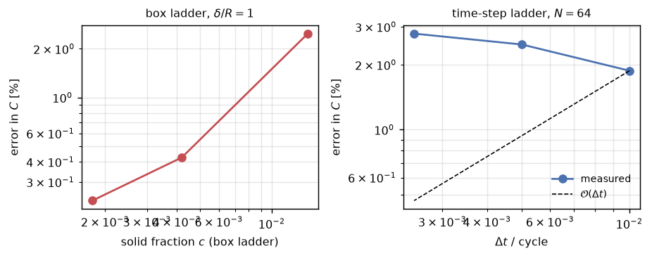
Why the steady calibration must not be applied here
The obvious move — divide the unsteady result by the steady box factor \(\lambda_{\text{box}}\) measured in Step 1 — is wrong, and wrong by a lot. A steady Stokeslet decays as \(1/r\), so its periodic images give the large correction Equation 2 describes (1.674 at \(c=\) 0.0141, i.e. a 65% effect). The oscillatory Stokeslet decays as \(e^{-r/\delta}/r\): at \(\delta/R = 1\) in this box, \(e^{-L/\delta} =\) 1.3e-03. There is essentially no viscous image correction to remove, and dividing by \(\lambda_{\text{box}}\) introduces a 40% error instead of removing one. Finite frequency screens the box.
Results
| claim | measured | reference |
|---|---|---|
| steady drag at \(c=\) 0.01414 | 1.67437 | Equation 2 1.69987 (-1.50%) |
| steady drag at \(c=\) 0.00177 (dilute) | 1.26559 | Equation 2 1.26748 (-0.15%) |
| steady drag, grid ladder at fixed \(c\) | -1.50% -> -1.43% | flat ⇒ converged |
| complex drag over \(\delta/R \in [0.5, 2.5]\) at \(L/R = 10\) | worst point 2.48%, best 0.25% | Stokes (1851) Equation 1 |
| error at the largest box ($L/R = $ 13.3, \(\delta/R = 1\)) | 0.23% — $C = $ +2.00245-1.21741i | +2.00000-1.22222i |
| box ladder, \(L/R\) 6.7 -> 13.3 | 2.48% -> 0.23% | converging |
| time-step ladder at \(N=64\) | 1.88% -> 2.79% | first order in \(\omega\Delta t\) |
The headline: the complex unsteady drag matches Stokes (1851) to 0.23% at \(\delta/R = 1\) in the largest box, with both the real and imaginary parts right — and the two residual error sources are separated rather than lumped, one shrinking with the box and one with the time step. The steady limit of the same setup reproduces the Hasimoto–Sangani–Acrivos periodic drag series to 0.15% at the same dilution, so the geometry and the reaction force are not the uncertain part.
Adapt this yourself
- Add rotation.
set_instance_motion(..., ang_vel=[0,0,W])gives the sphere a spin; the unsteady rotary drag has its own closed form and the same machinery measures it. - Go nonlinear. Raise the amplitude until \(A/R\) is no longer small, switch
set_advection(True)(the reaction budget carries explicit advection), and watch steady streaming appear — a second-order effect the linearised theory cannot see. - Change the shape. Any
peclet.core.geomtree can replace the sphere leaf; the drag is then a prediction rather than a check. - Move the geometry for real.
set_instance_transform+rebuild_geometrytranslates the body instead of only its boundary condition — the right route once \(A/R\) is not small, and the one case whererefresh_wall_velocityis not enough (it refuses, rather than running on stale geometry).
Reproduce this
PECLET_LOCAL_BUILD=/path/to/suite/flow/build_l3_cuda \
  quarto render examples/oscillating-sphere/index.qmd --execute
Roughly half an hour on an RTX 5080. Keep the pressure multigrid at depth ≥ 4: levels=1 leaves the coarse solve on the full grid and costs 920 ms/step instead of 19.5 at \(N=64\) on CUDA.
References
Hasimoto, H. 1959. “On the Periodic Fundamental Solutions of the Stokes Equations and Their Application to Viscous Flow Past a Cubic Array of Spheres.” Journal of Fluid Mechanics 5 (2): 317–28. https://doi.org/10.1017/S0022112059000222.
Sangani, A. S., and A. Acrivos. 1982. “Slow Flow Through a Periodic Array of Spheres.” International Journal of Multiphase Flow 8 (4): 343–60. https://doi.org/10.1016/0301-9322(82)90047-7.