import importlib.util, os, subprocess, sys
_local = os.environ.get("PECLET_LOCAL_BUILD")
if _local:
    for p in _local.split(os.pathsep):
        sys.path.insert(0, p)
elif importlib.util.find_spec("peclet") is None:
subprocess.run([sys.executable, "-m", "pip", "install", "-q", "peclet[cfd-dem]"], check=True)Bidisperse segregation: jetsam and flotsam in a fluidized bed
Fluidize a random mix of two grain species — small light nylon and large dense ceramic — and watch the bed sort itself: the nylon rises into a bubbling layer while the ceramic sinks to a near-static bottom. Online CFD–DEM with a true per-particle radius and mass, reproducing an MFIX-Exa qualitative benchmark and the Goldschmidt experiment.
coupling
cfd-dem
dem
flow
fluidization
segregation
polydisperse
gidaspow
benchmark
gpu
 This is an online CFD–DEM example (the two solvers exchange drag and void fraction every step), so it needs the
 peclet-coupling module — built from source, see Reproduce. It reproduces the Bidisperse segregation case from the MFIX-Exa qualitative benchmarks, which in turn follows the NETL rig and the classic experiments of Goldschmidt et al. (Goldschmidt et al. 2003).
What you’ll learn
The fluidized-bed example fluidized one kind of grain. Real beds are almost never monodisperse, and a mixture does something a single species cannot: it segregates. Give the bed two species that differ in size and density and the drag/weight balance sorts them vertically — the classic jetsam (sinks) / flotsam (floats) problem. This example shows how peclet handles a genuinely polydisperse bed:
- Assign every grain its own radius (
dem.set_scales) and its own mass (per-particle inverse mass), so the DEM contact solver and the CFD–DEM drag both see the real two-species mixture — not an averaged grain. - Fluidize a random mix of small light nylon (d = 3.19 mm, ρ = 1130 kg/m³) and large dense ceramic (d = 4.25 mm, ρ = 2580 kg/m³) with the Gidaspow drag law at a superficial velocity above both minimum-fluidization points.
- Measure the segregation dynamics — each species’ mean height versus time — and compare the sorted end-state to the MFIX-Exa benchmark and the Goldschmidt experiment.
import numpy as np, time
import matplotlib.pyplot as plt
from peclet import flow, dem
from peclet.coupling import CfdDem
plt.rcParams.update({"figure.dpi": 130, "font.size": 10, "axes.axisbelow": True,
                     "figure.facecolor": "white", "savefig.bbox": "tight"})
print("backends — flow:", flow.execution_space, " dem:", dem.execution_space)
backends — flow: Cuda dem: CudaThe setup — one small bed, two grain species
The rig is the NETL bidisperse bed: a square column 60.3 mm on a side, resolved (as in MFIX-Exa) on a deliberately coarse 8 × 8 × 24 grid — the CFD cell is about 2 particle diameters, which is all the unresolved point-particle model needs to define a void fraction. The solver runs in cell units (cell size h, time in seconds); every SI length becomes length / h, which preserves the drag physics exactly.
box_w        = 60.325e-3                       # square cross-section, m (NETL rig)
rho_g, mu_g  = 1.2, 1.8e-5                      # air
g            = 9.81
dp_n, rho_n  = 3.19e-3, 1130.0                 # nylon   — small, light (flotsam)
dp_c, rho_c  = 4.25e-3, 2580.0                 # ceramic — large, dense (jetsam)
U_si         = 2.0                             # superficial gas velocity, m/s (> both U_mf)

NX, NY, NZ   = 8, 8, 24
h            = box_w / NX                       # cell size = 7.54 mm
rp_n, rp_c   = dp_n/2/h, dp_c/2/h               # radii in cells
mu_c, g_c, U_c = mu_g/h**2, g/h, U_si/h         # SI -> cell units
m_n = rho_n*(4/3)*np.pi*rp_n**3                 # cell-consistent masses (radius in cells)
m_c = rho_c*(4/3)*np.pi*rp_c**3
print(f"cell h = {h*1e3:.2f} mm  (cell/d_nylon={h/dp_n:.1f}, cell/d_ceramic={h/dp_c:.1f})")
cell h = 7.54 mm (cell/d_nylon=2.4, cell/d_ceramic=1.8)
NoteMinimum fluidization sets the sorting
From the Wen & Yu correlation the two species fluidize at very different gas velocities — Umf ≈ 1.1 m/s for the nylon and ≈ 1.8 m/s for the ceramic. Driving at 2.0 m/s puts the gas well above the nylon’s threshold but only just above the ceramic’s: the nylon boils vigorously and rises, the ceramic barely lifts and stays near the distributor. That gap is the engine of segregation.
We fill the column with a random 50/50 mix on a jittered lattice, then let the DEM settle it into a packed bed under gravity — a well-mixed initial state, exactly as the benchmark prescribes.
rng = np.random.default_rng(3)
sp  = 1.05*2*rp_c
nxy = int((NX - 2*rp_c)/sp)
xs  = 1.0 + (np.arange(nxy)+0.5)*(NX-2)/nxy
pos, spec, k = [], [], 0
while len(pos) < 4200:
    z = rp_c + (k+0.5)*sp
    if z > 12: break
    for ix in range(nxy):
        for iy in range(nxy):
            pos.append((xs[ix], xs[iy], z)); spec.append(rng.integers(0, 2))
    k += 1
pos  = np.array(pos, np.float32); spec = np.array(spec)
pos[:, :2] += rng.uniform(-0.05, 0.05, (len(pos), 2)).astype(np.float32)
N     = len(pos)
is_n0 = spec == 0                               # nylon mask (insertion order)
rad   = np.where(is_n0, rp_n, rp_c).astype(np.float32)   # per-particle radius, cells
invm  = np.where(is_n0, 1/m_n, 1/m_c).astype(np.float32) # per-particle inverse mass
print(f"{N} grains — {is_n0.sum()} nylon + {(~is_n0).sum()} ceramic")
2880 grains — 1460 nylon + 1420 ceramicThe DEM carries the two species through per-particle scales and masses. A uniform base sphere is scaled grain-by-grain (set_scales), and the mass goes in as column 3 of the positions array. The box is five exact wall planes (a bouncy distributor floor plus four side walls) — no SDF, so nothing tunnels.
Important
set_scales comes after set_positions
The per-particle scale array is sized by the live particle count, which set_positions establishes. Call set_scales before setting positions and it applies to an empty bed (every grain keeps the base radius, and a bed of unit-radius grains explodes). The DEM keeps particle order stable across steps, so a species mask taken from get_scales() stays valid for the whole run.
d = dem.Simulation(int(1.3*N) + 64)
d.initialize(shape_type=1, radius=1.0); d.set_sphere_shape(1.0)
d.set_domain((0, 0, 0), (NX, NY, NZ)); d.enable_periodicity(False, False, False)
d.set_gravity(0, 0, -g_c)
d.set_material_params(0.9, 0.0, 0.15)           # restitution / friction
d.set_solver_iterations(10, 4)
dt = 2.0e-3; d.set_dt(dt/20)
d.add_plane((0, 0, 0), (0, 0, 1))                                       # distributor floor
d.add_plane((0, 0, 0), (1, 0, 0)); d.add_plane((NX, 0, 0), (-1, 0, 0))  # side walls
d.add_plane((0, 0, 0), (0, 1, 0)); d.add_plane((0, NY, 0), (0, -1, 0))
d.set_positions(np.c_[pos, invm])
d.set_scales(rad)                               # per-particle radius — AFTER set_positions
d.set_velocities(np.zeros((N, 3), np.float32))

for _ in range(1000): d.step(dt/20)             # settle the mix into a packed bed
sc   = d.get_scales()[:N]; is_n = sc < 0.5*(rp_n+rp_c)   # species mask, reorder-robust
print(f"settled — bed top z95 = {np.percentile(d.get_positions()[:N,2],95)*h*1e3:.0f} mm")
settled — bed top z95 = 42 mmThe gas side is the same box: a bottom inflow at the superficial velocity, a top outflow, and no-slip side walls. The coupling ties them together with the Gidaspow drag law and the volume-averaged (porous=True) continuity — the right model for a dense bed. Crucially, radius=rad hands the coupling the per-particle radius array, so the drag on each grain uses its own size.
s = flow.Solver(NX, NY, NZ)
s.set_rho(rho_g); s.set_mu(mu_c); s.set_dt(dt)
s.set_domain_bc(4, 2, 0.0, 0.0, U_c); s.set_domain_bc(5, 3)   # -z inflow, +z outflow
for f in (0, 1, 2, 3): s.set_domain_bc(f, 1)                  # no-slip sides
s.set_pressure_pcg(True, 40, 1e-6)

cpl = CfdDem(s, d, fluid_dt=dt, mu=mu_c, rho=rho_g, radius=rad, drag="gidaspow",
             dem_substeps=20, periodic=(False, False, False), move_particles=True, porous=True,
             eps_min=0.05, smooth_width=1.0)
ImportantGetting the coupling right on a coarse
cell ≈ 2 d grid
Three choices here are what make this bed fluidize and sort like the benchmark — each traceable to what MFIX does:
- The porous continuity must actually be enforced. The volume-averaged projection (
∂ε/∂t + ∇·(εu) = 0) rides the cut-cell pressure operator; a plain box with only domain BCs has none, and older versions silently fell back to no continuity constraint at all — the gas never accelerated to the interstitial velocityU/εin the bed, the slip the drag law saw was ~5× too small, and the bed refused to fluidize at any velocity.CfdDemnow installs an all-fluid pressure geometry automatically (andflowraises an error rather than degrade silently). With it, the imposed inlet velocity is the superficial velocity exactly: the inflow-face void fraction is pinned to 1 (the distributor contract), and the gas speeds up toU/εinside the packing. - No porosity floor. The solids fraction is clipped to \([0,1]\) only (
eps_min=0.05is a divide-by-zero guard, not a physical clamp). A dense packing’s true voidage sits near — and locally below — 0.4, and the Ergun drag scales like \(1/\varepsilon^{3}\): clamping ε up to 0.4 (the old default) under-predicts the drag ≈3× exactly where it must carry the bed. Small physical porosities are kept; if a drag law misbehaves there, change the correlation, not the ε. - Smooth the porosity, not the grid. With cells only ~2 diameters wide, a point-particle deposit gives a noisy ε.
smooth_width=1.0applies MFIX’s diffusive smoothing (DES_DIFFUSE_WIDTH): a volume-conserving Gaussian of ≈1 cell that decouples the porosity smoothing length from the mesh — the recipe the MFIX-Exa papers call crucial for grid-independent results.
The drag law itself is Gidaspow — exactly what the MFIX-Exa biseg benchmark uses, applied per-particle with each grain’s own diameter. (MFIX-Exa also offers the Beetstra–van der Hoef–Kuipers polydisperse correlation, but the benchmark does not use it, so neither do we.)
Fluidize and sort
Run three seconds of physical time, recording each species’ mean height as it goes and a handful of side-view snapshots.
NSTEP  = 1500
snap_at = {0: 0, NSTEP//4: 1, NSTEP//2: 2, NSTEP-1: 3}
snaps  = [None]*4; hist = []
t0 = time.time()
for i in range(NSTEP):
    cpl.step()
    P = np.asarray(d.get_positions())[:N]
    if i % 10 == 0:
        hist.append((i*dt, P[is_n, 2].mean()*h*1e3, P[~is_n, 2].mean()*h*1e3))
    if i in snap_at: snaps[snap_at[i]] = P.copy()
hist = np.array(hist)
print(f"{NSTEP} coupled steps ({NSTEP*dt:.1f} s) in {(time.time()-t0)/60:.1f} min")

def sideview(ax, P, title):
    m = np.abs(P[:,1] - NY/2) < 1.3                          # thin central y-slice
    ax.scatter(P[m&~is_n,0]*h*1e3, P[m&~is_n,2]*h*1e3, s=14, c="#d1495b", edgecolors="none", label="ceramic")
    ax.scatter(P[m& is_n,0]*h*1e3, P[m& is_n,2]*h*1e3, s=8,  c="#2e6f95", edgecolors="none", label="nylon")
    ax.set(title=title, xlim=(0, NX*h*1e3), ylim=(0, 150), aspect="equal", xlabel="x [mm]")

fig, ax = plt.subplots(1, 4, figsize=(10.5, 3.9))
for k, (i, lab) in enumerate([(0,"t = 0 (mixed)"), (NSTEP//4, f"t = {0.25*NSTEP*dt:.1f} s"),
                              (NSTEP//2, f"t = {0.5*NSTEP*dt:.1f} s"), (NSTEP-1, f"t = {NSTEP*dt:.1f} s")]):
    sideview(ax[k], snaps[k], lab)
ax[0].set_ylabel("height z [mm]"); ax[0].legend(loc="upper right", fontsize=8, framealpha=0.9)
plt.tight_layout()
1500 coupled steps (3.0 s) in 2.0 min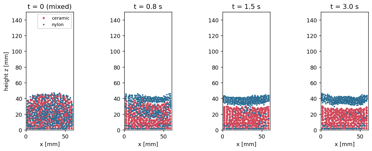
Two quantitative signatures pin the sort down. First, the divergence of the species’ mean heights: identical at t = 0 (fully mixed), they separate as the nylon floats up and the ceramic sinks — the strong oscillation is the bed slugging in a narrow column. Second, the final concentration profile: ceramic piles up near the distributor and vanishes above mid-bed, while nylon caps the top.
Vn, Vc = (4/3)*np.pi*rp_n**3, (4/3)*np.pi*rp_c**3
P = snaps[3]; zmm = P[:,2]*h*1e3
zedge = np.linspace(0, 90, 19); zc = 0.5*(zedge[:-1]+zedge[1:])
binvol = (NX*h*1e3)**2 * (zedge[1]-zedge[0])            # mm^3 per z-bin (full cross-section)
phi_n = np.histogram(zmm[is_n],  zedge)[0]*Vn*(h*1e3)**3/binvol
phi_c = np.histogram(zmm[~is_n], zedge)[0]*Vc*(h*1e3)**3/binvol

fig, ax = plt.subplots(1, 2, figsize=(9, 3.7))
ax[0].plot(hist[:,0], hist[:,1], color="#2e6f95", lw=2, label="nylon (small, light)")
ax[0].plot(hist[:,0], hist[:,2], color="#d1495b", lw=2, label="ceramic (large, dense)")
ax[0].fill_between(hist[:,0], hist[:,1], hist[:,2], color="0.85", zorder=0)
ax[0].set(xlabel="time [s]", ylabel="species mean height ⟨z⟩ [mm]", title="Segregation dynamics"); ax[0].legend()
ax[1].plot(phi_n, zc, color="#2e6f95", lw=2, marker="o", ms=3, label="nylon")
ax[1].plot(phi_c, zc, color="#d1495b", lw=2, marker="s", ms=3, label="ceramic")
ax[1].set(xlabel="solids volume fraction", ylabel="height z [mm]", title="Sorted bed (t = 3 s)"); ax[1].legend()
plt.tight_layout()
sep = hist[-1,1] - hist[-1,2]
print(f"final mean heights — nylon {hist[-1,1]:.0f} mm, ceramic {hist[-1,2]:.0f} mm; separation {sep:+.0f} mm")
final mean heights — nylon 33 mm, ceramic 15 mm; separation +18 mm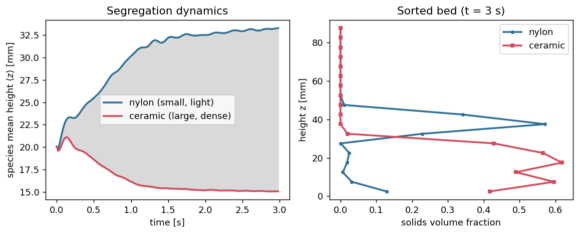
Results — peclet vs. MFIX-Exa vs. experiment
| Small/light species | Large/dense species | Segregation outcome | |
|---|---|---|---|
| Goldschmidt experiment (Goldschmidt et al. 2003) | rises, forms fluidized top layer | sinks toward distributor | strong, but takes several seconds |
| MFIX-Exa benchmark | fluidized nylon layer above | ceramic “essentially static” at bottom | segregates faster than experiment |
| peclet (this run) | nylon rises into bubbling layer | ceramic sinks to near-static base | same ordering; separation plateaus in ~1–2 s |
All three agree on the essential physics — nylon up, ceramic down — and peclet, like MFIX-Exa, segregates somewhat faster than the real bed. The MFIX-Exa notes attribute this to the coarse-grained, unresolved drag over-mobilizing the light species; the same coarse cell ≈ 2 d grid is in play here. The direction and steady sorted state are the benchmark’s qualitative target, and they reproduce cleanly.
Adapt this yourself
- Flip the ratio. Make the dense species also the smaller one (size and density fighting each other): segregation weakens and can invert — the competition Goldschmidt mapped out.
- Sweep the gas velocity. Just below the ceramic’s Umf the ceramic never mobilizes at all; far above both, vigorous bubbling remixes the bed. Segregation is strongest in the window between.
- Add a third species, or a continuous size distribution:
set_scalesand the per-particleradiusarray already take an arbitrary vector — nothing else changes. - Refine the grid. Push to
16 × 16 × 48(cell ≈ 1 d) to test how much the over-fast segregation is a coarse-grid artifact.
Reproduce this
# CPU (OpenMP) — flow + dem + the coupling module, built from source against a Kokkos prefix:
tools/bootstrap_deps.sh host-openmp
for m in flow dem coupling; do
  cmake -S $m -B $m/build -DCMAKE_PREFIX_PATH="$PWD/extern/install/host-openmp"; cmake --build $m/build -j
done
PECLET_LOCAL_BUILD="$PWD/flow/build:$PWD/dem/build:$PWD/coupling/build" \
  quarto render examples/bidisperse-segregation/index.qmd --execute
# GPU: point CMAKE_PREFIX_PATH at extern/install/nvidia-cuda (nvcc on PATH) and build the *_cuda_mphys dirs.
References
Goldschmidt, M. J. V., J. M. Link, S. Mellema, and J. A. M. Kuipers. 2003. “Digital Image Analysis Measurements of Bed Expansion and Segregation Dynamics in Dense Gas-Fluidised Beds.” Powder Technology 138 (2–3): 135–59. https://doi.org/10.1016/j.powtec.2003.09.003.