import importlib.util, os, subprocess, sys
_local = os.environ.get("PECLET_LOCAL_BUILD")
if _local:
    for p in _local.split(os.pathsep):
        sys.path.insert(0, p)
elif importlib.util.find_spec("peclet") is None:
subprocess.run([sys.executable, "-m", "pip", "install", "-q", "peclet"], check=True)Two fused spheres: the dumbbell against bispherical exactness
The touching two-sphere rigid body is one of the few composed shapes whose Stokes drag is known exactly — Stimson–Jeffery along the line of centres, Jeffrey–Onishi across it — and a CSG union of two sphere leaves reproduces the axial value to a tenth of a percent.
flow
IBM
csg
verification
analytic
drag
GPU
 GPU example — the frozen page reads correctly without a solver.
What you’ll learn
A rigid pair of equal touching spheres is the simplest composed particle there is — one CSG union of two sphere leaves — and, rarely for a composed shape, its unbounded Stokes drag is known exactly, from the classical bispherical-coordinate solutions. Per constituent sphere of radius \(a\) moving at \(U\):
\[ F_\parallel = 2\,\lambda_\parallel\, 6\pi\mu a U,\quad \lambda_\parallel = 0.64514 \qquad\text{(along the line of centres; Stimson & Jeffery 1926)} \] \[ F_\perp = 2\,\lambda_\perp\, 6\pi\mu a U,\quad \lambda_\perp = 0.72462 \qquad\text{(across it; Jeffrey & Onishi 1984)} \tag{1}\]
Each sphere carries less than the drag it would alone — the pair shelters itself — and by more along the line of centres than across it, which is why a settling dumbbell turns broadside-on. (The individual resistance functions diverge at contact; only these rigid-body sums are finite, which is why Kim & Karrila’s tables have no entry at contact and the numbers above come from the lubrication-complete series.) (Stimson and Jeffery 1926; Jeffrey and Onishi 1984)
The method is the non-spherical drag page’s, unchanged: measure the shape and an equal-volume sphere in the same periodic box and take the ratio, so the box cancels to leading order. With \(R_{\rm eq} = 2^{1/3} a\), the exact targets become
\[ K_\perp = \frac{2\lambda_\perp}{2^{1/3}} = 1.15026, \qquad K_\parallel = \frac{2\lambda_\parallel}{2^{1/3}} = 1.02410 . \tag{2}\]
import time
import numpy as np
import matplotlib.pyplot as plt
from peclet import flow as sdflow
from peclet.core import geom

plt.rcParams.update({"figure.dpi": 130, "font.size": 9, "axes.axisbelow": True,
                     "figure.facecolor": "white", "savefig.bbox": "tight"})
RHO, MU, F, DT = 1.0, 0.1, 1e-4, 1000.0
A = 6.0
REQ = A * 2 ** (1 / 3)
KI_I, KI_R = 2, 17

def run(build, N, label, tol=1e-7, maxit=3000):
    b = geom.SceneBuilder()
    root = build(b)
    ni, nr, _, _ = b.encode()
    ii = np.zeros((1, KI_I), dtype=np.int32); ii[0] = (root, -1)
    ir = np.zeros((1, KI_R)); ir[0, 0:3] = (0.5 * N,) * 3; ir[0, 6] = 1.0; ir[0, 7] = 1.0
    s = sdflow.Solver(N, N, N)
    s.set_rho(RHO); s.set_mu(MU); s.set_dt(DT); s.set_advection(False)
    s.set_velocity_solver_params(80); s.set_pressure_solver_params(20)
    s.set_pressure_multigrid(True, levels=4)
    s.set_scene(np.asarray(ni, np.int32), np.asarray(nr, float), ii.ravel(), ir.ravel(),
                periodic=True)
    s.set_solid_from_scene(True)
    s.set_body_force(F, 0.0, 0.0)
    nc = s.fluid_momentum_cells()[0]
    prev, it, t0 = 0.0, 0, time.time()
    while it < maxit:
        s.step(); it += 1
        um = float(np.asarray(s.get_u()).sum()) / nc
        if it > 5 and abs(um - prev) < tol * abs(um):
            break
        prev = um
    Fh = float(np.asarray(s.hydro_force_torque_reaction())[0][0][0])
    lam = Fh / (6 * np.pi * MU * REQ * um)
    print("  %-26s N=%3d  lambda=%.5f   (%d steps, %3.0f s)"
          % (label, N, lam, it, time.time() - t0))
    return lam

SPHERE    = lambda b: b.add_leaf("sphere", [REQ])
BROADSIDE = lambda b: b.add_union(b.add_leaf("sphere", [A], translation=[0, -A, 0]),
                                  b.add_leaf("sphere", [A], translation=[0, +A, 0]))
EDGE_ON   = lambda b: b.add_union(b.add_leaf("sphere", [A], translation=[-A, 0, 0]),
                                  b.add_leaf("sphere", [A], translation=[+A, 0, 0]))
K_PERP_EX = 2 * 0.72462 / 2 ** (1 / 3)
K_PAR_EX  = 2 * 0.64514 / 2 ** (1 / 3)
Kokkos::OpenMP::initialize WARNING: OMP_PROC_BIND environment variable not set
In general, for best performance with OpenMP 4.0 or better set OMP_PROC_BIND=spread and OMP_PLACES=threads
For best performance with OpenMP 3.1 set OMP_PROC_BIND=true
For unit testing set OMP_PROC_BIND=false
The measurement, in two boxes
The flow is along \(x\): EDGE_ON puts the line of centres along the flow (\(\lambda_\parallel\)), BROADSIDE across it (\(\lambda_\perp\)). The second box is the honest error bar: the non-spherical drag page measured that elongated bodies do not block a periodic box the way an equal-volume sphere does, so the ratio’s residual shifts with the box — and it shifts most for the orientation where the body is longest transverse to the flow.
rows = []
for N in (96, 128):
    ls = run(SPHERE, N, "equal-volume sphere")
    lb = run(BROADSIDE, N, "dumbbell broadside")
    le = run(EDGE_ON, N, "dumbbell edge-on")
    rows.append((N, lb / ls, le / ls))
    print("  N=%3d (c=%.2e):  K_perp = %.5f (%+.2f%%)   K_par = %.5f (%+.2f%%)"
          % (N, (4 / 3) * np.pi * REQ ** 3 / N ** 3,
             lb / ls, 100 * (lb / ls / K_PERP_EX - 1),
             le / ls, 100 * (le / ls / K_PAR_EX - 1)))
equal-volume sphere N= 96 lambda=1.27708 (2267 steps, 213 s)
dumbbell broadside N= 96 lambda=1.53247 (1930 steps, 164 s)
dumbbell edge-on N= 96 lambda=1.30881 (2219 steps, 120 s)
N= 96 (c=2.05e-03): K_perp = 1.19998 (+4.32%) K_par = 1.02485 (+0.07%)
equal-volume sphere N=128 lambda=1.19961 (3000 steps, 413 s)
dumbbell broadside N=128 lambda=1.41854 (3000 steps, 527 s)
dumbbell edge-on N=128 lambda=1.22999 (3000 steps, 487 s)
N=128 (c=8.63e-04): K_perp = 1.18250 (+2.80%) K_par = 1.02532 (+0.12%)Code
fig, ax = plt.subplots(figsize=(5.6, 3.2))
x = np.arange(2)
w = 0.3
for k, (N, kb, ke) in enumerate(rows):
    ax.bar(x + (k - 0.5) * w, [kb, ke], w * 0.9,
           color=["#4c72b0", "#8fa9c8"][k], label="$N=%d$" % N)
ax.plot([x[0]], [K_PERP_EX], "k*", ms=13, zorder=5)
ax.plot([x[1]], [K_PAR_EX], "k*", ms=13, zorder=5, label="exact (bispherical)")
ax.set_xticks(x); ax.set_xticklabels(["broadside\n$K_\\perp$", "edge-on\n$K_\\parallel$"])
ax.set_ylabel(r"$K = F / F_{\rm eq.vol.\ sphere}$")
ax.set_ylim(0.95, 1.25)
ax.legend(fontsize=8, frameon=False); ax.grid(axis="y", alpha=0.3)
plt.show()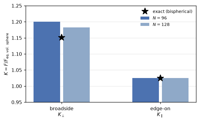
Results
| claim | measured | exact |
|---|---|---|
| edge-on \(K_\parallel\) (\(N=128\)) | 1.02532 | 1.02410 (+0.12%) |
| broadside \(K_\perp\), \(N = 96 \to 128\) | 1.19998 -> 1.18250 | 1.15026 — the residual shrinks with the box |
| the settling anisotropy \(K_\perp/K_\parallel\) (\(N=128\)) | 1.1533 | 1.1232 |
The contact point itself deserves a sentence: the CSG union’s SDF is exact everywhere for this shape, including the non-smooth neck at contact, and the aperture-based cut cells never need the (divergent) individual resistance functions — the discrete body is the rigid pair from the start, which is precisely the object the bispherical sums describe.
Adapt this yourself
- Unequal spheres.
translation=[±a₁,…]with two radii gives the asymmetric doublet; the bispherical machinery covers it, and the drag becomes a prediction with a literature check. - Let it settle freely. With
scene_particle’s principal-frame inertia, the same body drops into the resolved CFD-DEM loop; the broadside-vs-edge-on ratio above is why it turns broadside-on, and withapply_torque=True(see the Jeffery orbit) the reorientation itself is simulated rather than argued. - Separate them. Two distinct sphere instances at increasing gap traces the full interaction curve down from contact — the resolved version of the mobility tables.
Reproduce this
PECLET_LOCAL_BUILD=/path/to/suite/flow/build_l3_cuda:/path/to/suite/core/python/build_geom \
  quarto render examples/dumbbell-drag/index.qmd --execute
References
Jeffrey, D. J., and Y. Onishi. 1984. “Calculation of the Resistance and Mobility Functions for Two Unequal Rigid Spheres in Low-Reynolds-Number Flow.” Journal of Fluid Mechanics 139: 261–90. https://doi.org/10.1017/S0022112084000355.
Stimson, M., and G. B. Jeffery. 1926. “The Motion of Two Spheres in a Viscous Fluid.” Proceedings of the Royal Society of London. Series A 111 (757): 110–16. https://doi.org/10.1098/rspa.1926.0053.