import importlib.util, os, subprocess, sys
_local = os.environ.get("PECLET_LOCAL_BUILD")
if _local:
    for p in _local.split(os.pathsep):
        sys.path.insert(0, p)
elif importlib.util.find_spec("peclet") is None:
subprocess.run([sys.executable, "-m", "pip", "install", "-q", "peclet"], check=True)Developing channel flow: from a flat inlet to Poiseuille
A uniform stream enters a channel and relaxes into the parabolic profile — the classic entrance-region problem, with inflow/outflow boundaries.
flow
inflow-outflow
boundary-conditions
verification
 Runs on a free Colab CPU runtime — the first cell installs
 peclet from PyPI.
What you’ll learn
How to set an inflow/outflow problem in peclet.flow and watch a boundary layer grow. A uniform stream enters a plane channel; the no-slip walls brake the fluid near them, a boundary layer thickens downstream, and — once the layers from the two walls merge — the flow becomes fully developed plane Poiseuille flow. This entrance region is a staple of every internal-flow course, and it is the natural first test of the inflow/outflow machinery (a Dirichlet-velocity inlet, a zero-gradient outflow, and the projection that lets mass leave the domain).
Setup
A channel of height \(H\) and length \(L\): uniform inlet velocity \(U\) on the \(-x\) face (set_domain_bc(0, 2, U, 0, 0)), an outflow on \(+x\) (type 3), and no-slip walls on \(\pm y\) (type 1). No immersed solid — the domain is all fluid with boundary-condition pressure faces (set_pressure_geometry). The Reynolds number is \(\mathrm{Re} = U H/\nu\), and the entrance length scales as \(L_e \sim 0.04\,\mathrm{Re}\,H\).
import numpy as np
import matplotlib.pyplot as plt
from peclet import flow

plt.rcParams.update({"figure.dpi": 130, "font.size": 10, "axes.grid": True,
                     "grid.alpha": 0.3, "axes.axisbelow": True,
                     "figure.facecolor": "white", "savefig.bbox": "tight"})
BLUE, RED = "#1f77b4", "#d62728"
Solve to steady state
def solve_developing(L=120, H=24, Re=60.0, U=1.0, nz=4, dt=0.5, max_steps=5000):
    nu = U * H / Re
    s = flow.Solver(L, H, nz)
    s.set_rho(1.0); s.set_mu(nu); s.set_dt(dt); s.set_advection(True)
    s.set_domain_bc(0, 2, U, 0.0, 0.0)      # -x uniform inflow (Dirichlet velocity)
    s.set_domain_bc(1, 3)                    # +x outflow (zero-gradient u, p=0)
    s.set_domain_bc(2, 1); s.set_domain_bc(3, 1)   # -y, +y no-slip walls
    s.set_velocity_solver_params(60)
    s.set_pressure_multigrid(True, levels=8)
    s.set_pressure_solver_params(80)
    s.set_pressure_geometry(np.full((L, H, nz), 1e30))   # all-fluid + BC pressure faces
    prev = 0.0
    for it in range(max_steps):
        s.step()
        if it % 100 == 99:
            m = float(s.get_u()[L - 4, H // 2, nz // 2])
            if it > 600 and abs(m - prev) < 2e-5 * (abs(m) + 1e-30):
                break
            prev = m
    return dict(L=L, H=H, Re=Re, U=U, nu=nu, u=s.get_u()[:, :, nz // 2],
                p=s.get_p()[:, :, nz // 2], steps=it + 1, div=float(s.max_open_divergence()))

r = solve_developing()
L, H, U = r["L"], r["H"], r["U"]
u = r["u"]
Umean = u[L - 4, :].mean()
print(f"Re={r['Re']:.0f}  L={L}  H={H}  steady in {r['steps']} steps   "
      f"outlet u_max/U_mean = {u[L-4].max()/Umean:.4f} (Poiseuille 1.5)   max divergence = {r['div']:.1e}")
# mass conservation: streamwise flux at inlet vs outlet
flux_in, flux_out = u[2, :].sum(), u[L - 3, :].sum()
print(f"mass conservation: |flux_out - flux_in|/flux_in = {abs(flux_out-flux_in)/flux_in:.2e}")
Re=60 L=120 H=24 steady in 700 steps outlet u_max/U_mean = 1.4934 (Poiseuille 1.5) max divergence = 1.9e-08
mass conservation: |flux_out - flux_in|/flux_in = 0.00e+00The boundary layer growing
The streamwise velocity: a flat inlet on the left, thickening wall boundary layers, and the fully developed parabola on the right. The white combs are the local \(u(y)\) profiles.
x = np.arange(L); y = np.arange(H)
fig, ax = plt.subplots(figsize=(9, 2.6))
pc = ax.pcolormesh(x, y, u.T, cmap="viridis", shading="auto")
stations = [int(f * L) for f in (0.02, 0.12, 0.3, 0.55, 0.95)]
for xi in stations:                                  # overlay u(y) as a comb at each station
    ax.plot(xi + u[xi] / U * 10, y, color="white", lw=1.2)
    ax.axvline(xi, color="white", ls=":", lw=0.5, alpha=0.6)
ax.set(title=f"Developing channel flow, Re={r['Re']:.0f}", xlabel="x", ylabel="y", aspect="equal")
ax.grid(False)
fig.colorbar(pc, ax=ax, fraction=0.02, pad=0.02, label="u")
plt.show()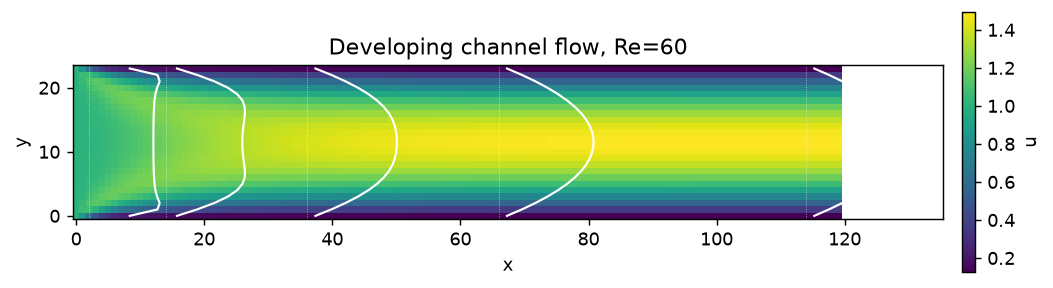
Profiles at stations and the centreline development
Normalised by the inlet speed, the profile starts flat (\(u/U=1\)) and relaxes to the parabola with peak \(1.5\,U_\text{mean}\). The centreline velocity accelerates (mass is conserved as the near-wall fluid slows) until it plateaus — the end of the entrance region.
yc = (np.arange(H) + 0.5) / H
parab = 6 * Umean * yc * (1 - yc)                     # developed Poiseuille (U_mean-normalised)

fig, (a0, a1) = plt.subplots(1, 2, figsize=(9.2, 3.8))
cols = plt.cm.viridis(np.linspace(0.15, 0.9, len(stations)))
for xi, c in zip(stations, cols):
    a0.plot(u[xi] / U, yc, color=c, label=f"x/L={xi/L:.2f}")
a0.plot(parab / U, yc, "k--", lw=1, label="parabola")
a0.set(xlabel="u / U", ylabel="y / H", title="profiles develop to Poiseuille"); a0.legend(fontsize=7)

cl = u[:, H // 2] / U
a1.plot(x / H, cl, "-", color=BLUE, label="centreline u/U")
a1.axhline(1.5 * Umean / U, ls="--", color=RED, label="1.5·U_mean/U")
target = 0.99 * 1.5 * Umean
Le = next((xi for xi in x if cl[xi] * U >= target), L) / H
a1.axvline(Le, color="0.4", ls=":", label=f"L_e/H≈{Le:.1f}")
a1.set(xlabel="x / H", ylabel="centreline u / U", title="entrance-region development"); a1.legend(fontsize=8)
fig.tight_layout()
plt.show()

dpdx = (r["p"][L // 2, H // 2] - r["p"][L - 8, H // 2]) / (L - 8 - L // 2)
print(f"entrance length L_e/H ≈ {Le:.1f}  (correlation 0.04·Re ≈ {0.04*r['Re']:.1f})")
print(f"developed dp/dx = {dpdx:.3e}   vs analytic -12·μ·U_mean/H² = {-12*r['nu']*Umean/H**2:.3e}")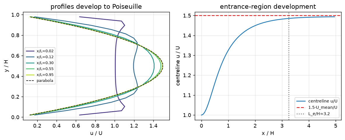
entrance length L_e/H ≈ 3.2  (correlation 0.04·Re ≈ 2.4)
developed dp/dx = 8.535e-03   vs analytic -12·μ·U_mean/H² = -8.333e-03
The takeaway
- The inflow/outflow BCs reproduce the textbook entrance-region development: a flat inlet becomes plane Poiseuille, with outlet \(u_\max/U_\text{mean}\to1.5\), machine-level mass conservation, and a developed pressure gradient matching \(-12\mu U_\text{mean}/H^2\).
- The entrance length follows the \(L_e\sim0.04\,\mathrm{Re}\,H\) scaling.
- Unlike the body-force Poiseuille example (periodic, fully developed by construction), here the profile is an output of the inflow/outflow solve.
Adapt this yourself
- Change Re. Higher
Relengthens the entrance region (∝ Re); makeLlonger to contain it. - Non-uniform inlet. Use
set_domain_bc_profileto prescribe an arbitrary inlet profile (e.g. the top-hat-with-shear of a real duct). - Add a body inside. Drop an SDF obstacle in with
set_solid(sdf, cutcell_pressure=True)— the inflow/outflow + immersed-body path (see the cylinder vortex-street example).
Reproduce this
pip install peclet            # needs peclet-flow >= 0.2.1 (inflow/outflow)
quarto render examples/developing-channel/index.qmd --execute
# ...or against a local source build:
PECLET_LOCAL_BUILD=/path/to/suite/flow/build_mpi OMP_NUM_THREADS=6 \
  quarto render examples/developing-channel/index.qmd --execute