# Makes this notebook run out-of-the-box on Colab/Binder. A real user just needs the
# published package; this installs it on first run. Authors can instead point at a
# local source build of the suite with the PECLET_LOCAL_BUILD env var.
import importlib.util, os, subprocess, sys
_local = os.environ.get("PECLET_LOCAL_BUILD")
if _local:
    sys.path.insert(0, _local)                                  # local source build
elif importlib.util.find_spec("peclet") is None:
subprocess.run([sys.executable, "-m", "pip", "install", "-q", "peclet"], check=True)Advecting an interface: Zalesak, LeVeque, and a conservation floor at 1e-14
The two classical volume-of-fluid transport tests, run on the production solver — and the number that only a geometric scheme can put on the table.
flow
vof
two-phase
advection
verification
 The \(32^3\) and \(64^3\) rungs run on a free Colab CPU runtime; the \(128^3\) rung wants a GPU build.
What you’ll learn
Before a two-phase solver can be trusted with surface tension, buoyancy or a wall, it has to be trusted with the one thing it does every step: move a sharp interface through a fixed grid without inventing or destroying liquid. This page runs the two benchmarks the volume-of-fluid literature has used for that since the 1970s, on peclet’s production transport scheme — Weymouth–Yue split geometric advection (Weymouth and Yue 2010) with a piecewise-linear (PLIC) reconstruction — and reports four things:
- Zalesak’s slotted disc (Zalesak 1979) after one solid-body revolution: a relative shape error of \(2.8\times10^{-2}\) at \(100^2\), sitting inside the published spread for this exact disc.
- LeVeque’s 3-D deformation field (LeVeque 1996) with reversal at \(T=3\): the shape error falls at order 2.16 from \(64^3\) to \(128^3\), the asymptotic PLIC rate.
- The conservation floor. Volume drift over 3200 steps at \(128^3\) is \(5.7\times10^{-14}\) — and that is not a discretization error at all. It is the round-off in the velocity field’s own discrete divergence, which is why the number goes down when you improve the projection and not when you refine the grid.
- Through an immersed solid. The same transport, openness-weighted, carries a liquid slab through a resolved sphere packing on a frozen Stokes velocity: drift \(-5.0\times10^{-12}\) against a projection residual of \(3.9\times10^{-11}\), with the colour in solid cells exactly zero.
Plus the two failure modes worth knowing about before you meet them: what happens when the prescribed velocity is only analytically divergence-free, and where the Courant limit of a geometric scheme actually is (it is \(1/4\) in 3-D, not \(1/2\)).
The conclusion to carry away: with a geometric VoF, conservation is an algebraic identity, not an accuracy claim — so the honest error bar on the volume is set by the pressure solve upstream of it, and the honest error bar on the shape is second order.
The problem
The colour function \(C(\mathbf{x},t)\in[0,1]\) is the liquid volume fraction of a cell. Under a prescribed incompressible velocity it obeys
\[ \frac{\partial C}{\partial t} + \nabla\!\cdot(C\,\mathbf{u}) = C\,\nabla\!\cdot\mathbf{u} , \tag{1}\]
where the right-hand side is identically zero in the continuum but not in the discrete equation, and that is the whole story of this page.
peclet integrates Equation 1 by operator splitting: three directional sweeps per step, each one clipping a slab of thickness \(a_f = u_f\,\Delta t/h\) off the donor cell’s reconstructed PLIC polyhedron and handing the liquid part of it to the acceptor — the split-advection construction of Aulisa et al. (2007) in three-dimensional Cartesian geometry. A directionally split scheme compresses and expands the cell volume between sweeps, so each sweep must add back a dilation term. Weymouth & Yue’s contribution (Weymouth and Yue 2010) is the observation that if that term is
\[ +\,c^{\,n}_i \left(a_{f^+} - a_{f^-}\right), \qquad c^{\,n}_i = H\!\left(C^n_i - \tfrac12\right)\in\{0,1\}, \tag{2}\]
with the flag \(c^{\,n}_i\) frozen at the start of the step and reused unchanged by all three sweeps, then summing the update over the whole grid telescopes: every flux appears twice with opposite signs, and what is left is
\[ \sum_i \Delta C_i \;=\; \sum_i c^{\,n}_i \sum_f \pm\,a_f \;=\; \frac{\Delta t}{h}\sum_i c^{\,n}_i \,(\nabla\!\cdot\mathbf{u})_i . \tag{3}\]
Two consequences, and they are the reason this page exists:
- Conservation is exact — algebraically, not asymptotically — provided the discrete divergence on the right of Equation 3 vanishes. Not the analytic divergence: the discrete one, the actual sum of the actual face values the scheme actually uses. Hand the scheme a velocity whose discrete divergence is \(O(h^2)\) — which is what a carelessly sampled analytic field generally gives you — and the conservation floor is \(O(h^2)\) too, ten orders above where it belongs.
- Conservation is independent of boundedness. Equation 3 holds whatever \(C\) does. An over-CFL run therefore does not lose volume; it loses \(0\le C\le1\). That failure is quiet, which is why the solver carries a hard Courant cap rather than trusting a volume check to catch it.
The shape error we report is the metric used across the VoF literature,
\[ \frac{L_1}{V} = \frac{\sum_i \lvert C_i - C^{\rm exact}_i\rvert}{\sum_i C^{\rm exact}_i} , \tag{4}\]
with \(C^{\rm exact}\) the initial field — both benchmarks are constructed so the exact solution at the final time is the initial condition, which removes the sampling error of the initial condition from the metric entirely.
import time
import numpy as np
import matplotlib.pyplot as plt
from peclet import flow

plt.rcParams.update({"figure.dpi": 130, "font.size": 10, "axes.grid": True,
                     "grid.alpha": 0.3, "axes.axisbelow": True,
                     "figure.facecolor": "white", "savefig.bbox": "tight"})
BLUE, RED, GREY, GREEN = "#1f77b4", "#d62728", "0.80", "#2ca02c"
PI = np.pi
NoteThe one API call this page is built on
advect_vof(dt) advances the colour field once with the solver’s current face velocity and does nothing else — no momentum, no pressure, no closures. That is what makes a transport benchmark a statement about the transport scheme. It throws if the current velocity is not discretely divergence-free to \(10^{-10}\) (Equation 3 again), so a prescribed field has to earn its way in.
1. Zalesak’s slotted disc
The oldest interface-advection test there is (Zalesak 1979): a disc with a rectangular notch cut out of it, carried once around a periodic box by rigid-body rotation. After one revolution the exact solution is the initial condition, and every corner the scheme has rounded off, every wisp it has shed and every bit of the slot it has healed shut shows up in Equation 4. It is a hard test for a piecewise-linear reconstruction, because the notch has four corners and PLIC resolves a corner with one plane per cell.
peclet works in cell units (\(h=1\)), so we use the canonical setup at \(100\times100\) in-plane resolution and 4 cells of thickness: disc of radius 15 centred at \((50, 75)\), slot of half-width 2.5 reaching up to \(y=85\), rotation about the box centre.
def zalesak_fractions(nx, ny, nz, c, r, sw, stop, nsub=64):
    """Liquid fraction of a slotted disc by nsub x nsub midpoint subsampling in (x,y),
    uniform in z. Cell units: cell (i,j) spans [i,i+1] x [j,j+1]."""
    w = 1.0 / nsub
    xs = (np.arange(nx)[:, None] + (np.arange(nsub)[None, :] + 0.5) * w).ravel()
    ys = (np.arange(ny)[:, None] + (np.arange(nsub)[None, :] + 0.5) * w).ravel()
    frac = np.zeros((nx, ny))
    chunk = max(1, nx // 10)
    for i0 in range(0, nx, chunk):                    # chunked: 100*64 squared is a big temporary
        i1 = min(nx, i0 + chunk)
        dx = xs[i0 * nsub:i1 * nsub][:, None] - c[0]
        Y = ys[None, :]
        inside = ((dx**2 + (Y - c[1])**2) < r * r) & ~((np.abs(dx) < sw) & (Y < stop))
        frac[i0:i1] = inside.reshape(i1 - i0, nsub, ny, nsub).mean(axis=(1, 3))
    return np.asfortranarray(np.repeat(frac[:, :, None], nz, axis=2))

NX, NY, NZ = 100, 100, 4
C0_zal = zalesak_fractions(NX, NY, NZ, (50.0, 75.0), 15.0, 2.5, 85.0)
r, sw, dy = 15.0, 2.5, 85.0 - 75.0                       # radius, slot half-width, slot reach
slot = 2 * (sw * np.sqrt(r*r - sw*sw) / 2 + r*r/2 * np.arcsin(sw/r)) + 2 * sw * dy
print(f"in-plane liquid area {C0_zal[:, :, 0].sum():.4f} cells^2   "
      f"vs exact (disc - slot) {PI*r*r - slot:.4f}")
in-plane liquid area 582.2129 cells^2 vs exact (disc - slot) 582.2070The velocity is the second half of the setup, and it is where a staggered code wants care. flow stores u(i,j,k) on the low \(x\)-face of cell \((i,j,k)\), i.e. at \(\big(i,\ j+\tfrac12,\ k+\tfrac12\big)\), and likewise for \(v\) and \(w\) on their own axes. Sampling \(\mathbf{u} = \omega\,(-(y-c_y),\ x-c_x,\ 0)\) at those points makes the discrete divergence vanish bitwise and for free: \(u\) does not depend on \(i\) and \(v\) does not depend on \(j\), so every 1-D difference in Equation 3 is a difference of two identical doubles.
def rotation_velocity(nx, ny, nz, cx, cy, omega):
    """Rigid-body rotation on flow's staggered faces: u on the LOW x-face of each cell,
    v on the LOW y-face. Discrete divergence is exactly zero (identical doubles differenced)."""
    j = np.arange(ny)[None, :, None]
    i = np.arange(nx)[:, None, None]
    u = np.broadcast_to(-omega * ((j + 0.5) - cy), (nx, ny, nz))    # face x = i, y-centre
    v = np.broadcast_to(omega * ((i + 0.5) - cx), (nx, ny, nz))     # face y = j, x-centre
    return (np.asfortranarray(u.astype(float)), np.asfortranarray(v.astype(float)),
            np.asfortranarray(np.zeros((nx, ny, nz))))
Driving the solver is four calls. set_pressure_geometry with an all-positive SDF puts the solver on its cut-cell operator with every face fully open — no solid, but it is what makes max_open_divergence() a live diagnostic (§3), and it is the same operator the immersed-solid run in §5 uses. set_state uploads the prescribed faces, and then advect_vof is called in a bare loop.
STEPS_ZAL = 1000                    # the published setup: one revolution in 1000 steps
def run_zalesak(steps=STEPS_ZAL, cfl_cap=0.5, C0=C0_zal):
    omega = 2.0 * PI / steps        # dt = 1 cell-time, so `steps` steps is one revolution
    u, v, w = rotation_velocity(NX, NY, NZ, 50.0, 50.0, omega)
    s = flow.Solver(NX, NY, NZ)
    s.set_rho(1.0); s.set_mu(1.0); s.set_dt(1.0)
    s.set_pressure_geometry(np.full((NX, NY, NZ), 10.0, order="F"))   # all-fluid, faces open
    s.enable_vof()
    s.set_vof(C0)
    s.set_state(u, v, w)
    s.set_vof_cfl_limit(cfl_cap)
    d0, div, cfl = s.vof_diagnostics(), s.max_open_divergence(), 0.0
    for _ in range(steps):
        s.advect_vof(1.0)
        cfl = max(cfl, s.vof_last_courant())
    d1, C1 = s.vof_diagnostics(), s.get_vof()
    l1 = np.abs(C1 - C0).sum()
    return dict(C=C1, l1=l1, rel=l1 / C0.sum(), E1=l1 / (NX * NY * NZ), cfl=cfl, div=div,
                drift=(d1["sum"] - d0["sum"]) / d0["sum"],
                minC=d1["min"], maxC=d1["max"], mixed=d1["mixed"], wisps=d1["wisps"])

t0 = time.time()
zal = run_zalesak()
print(f"one revolution, {STEPS_ZAL} steps, {NX}x{NY} in-plane   ({time.time()-t0:.1f} s)")
print(f"  L1/V (relative shape error)   {zal['rel']:.4e}")
print(f"  E1  (per-cell mean, 2-D)      {zal['E1']:.4e}")
print(f"  volume drift                  {zal['drift']:.3e}")
print(f"  C range                       [{zal['minC']:.3e}, {zal['maxC']:.6f}]"
      f"   mixed {zal['mixed']}  wisps {zal['wisps']}")
print(f"  max interface Courant number  {zal['cfl']:.4f}"
      f"   |  prescribed max|div(open u)| {zal['div']:.1e}")
one revolution, 1000 steps, 100x100 in-plane (3.1 s)
L1/V (relative shape error) 2.7835e-02
E1 (per-cell mean, 2-D) 1.6206e-03
volume drift 0.000e+00
C range [-3.778e-17, 1.000000] mixed 716 wisps 20
max interface Courant number 0.3110 | prescribed max|div(open u)| 0.0e+00Ci, Cf = C0_zal[:, :, 2], zal["C"][:, :, 2]
fig, axes = plt.subplots(1, 3, figsize=(8.4, 3.0))
for ax, (F, t) in zip(axes[:2], [(Ci, "initial $C$"), (Cf, f"after one revolution")]):
ax.imshow(F.T, origin="lower", cmap="Blues", vmin=0, vmax=1,
extent=(0, NX, 0, NY), interpolation="nearest")
ax.set(title=t, xlim=(28, 72), ylim=(55, 95)); ax.grid(False)
axes[2].contourf(np.arange(NX) + .5, np.arange(NY) + .5, Ci.T, [0.5, 1.5],
colors=["0.86"])
axes[2].contour(np.arange(NX) + .5, np.arange(NY) + .5, Cf.T, [0.5],
colors=[BLUE], linewidths=1.5)
axes[2].set(title="exact (grey fill) vs transported", xlim=(28, 72), ylim=(55, 95), aspect=1)
axes[2].grid(False)
for ax in axes:
ax.set_xlabel("x [cells]")
axes[0].set_ylabel("y [cells]")
plt.tight_layout(); plt.show()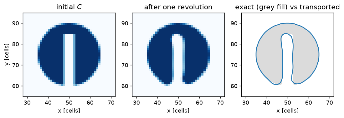
The headline: 2.78e-02. Published values on this identical disc and metric — Xie & Xiao’s Table 5 at \(N=100\) — run from \(1.55\times10^{-2}\) (THINC-scaling) through \(1.61\times10^{-2}\) (MTHINC) and \(2.61\times10^{-2}\) (UMTHINC) to \(3.22\times10^{-2}\) (THINC/QQ). A linear PLIC belongs at the upper end of that band and lands there: the schemes below it buy their margin with a quadratic or hyperbolic-tangent interface representation bought specifically to hold this slot’s corners. The second anchor, Cassinelli et al.’s per-cell mean \(E_1\), reads 1.621e-03 here, inside their PLIC band.
And the volume drift is 0.0e+00 — with a solid-body rotation whose discrete divergence is a bitwise zero, Equation 3 has nothing to add and the total colour is a fixed point of 1000 steps of a nonlinear geometric scheme.
2. LeVeque’s 3-D deformation field, with reversal
The rotation test is kind: the flow is rigid, so a scheme that merely translates well does well. LeVeque’s deformation field (LeVeque 1996) is not kind. It stretches a sphere into a thin, hollow, spiralling sheet — several cells thick at \(32^3\), and at maximum stretch genuinely under-resolved — then reverses in time (\(\cos(\pi t/T)\), \(T=3\)) and un-stretches it. The exact solution at \(t=T\) is again the initial sphere, so the error is everything the scheme lost while the interface was thinner than the mesh.
\[ \begin{aligned} u &= \phantom{-}2\sin^2(\pi x)\,\sin(2\pi y)\,\sin(2\pi z)\;\cos(\pi t/T),\\ v &= -\sin(2\pi x)\,\sin^2(\pi y)\,\sin(2\pi z)\;\cos(\pi t/T),\\ w &= -\sin(2\pi x)\,\sin(2\pi y)\,\sin^2(\pi z)\;\cos(\pi t/T). \end{aligned} \tag{5}\]
Sampling it so that it is discretely solenoidal
Equation 5 is analytically divergence-free. That is not the property Equation 3 needs. The property it needs is that the sum of the face values the scheme uses vanishes, per cell, in floating point — and the general way to guarantee that is to never write the velocity down at all. Write down an edge vector potential instead and take its discrete curl:
\[ \mathbf{A} = \Big(0,\; -\tfrac{\sin^2\!\pi x \,\sin^2\!\pi z}{\pi}\sin 2\pi y,\; \phantom{-}\tfrac{\sin^2\!\pi x \,\sin^2\!\pi y}{\pi}\sin 2\pi z\Big)\cos(\pi t/T), \tag{6}\]
whose continuum curl is exactly Equation 5. A discrete curl on the staggered mesh is divergence-free by construction: each edge value enters two face differences with opposite signs, and the divergence sum cancels them term by term in IEEE arithmetic, not merely to \(O(h^2)\).
def sin2(t):
    return np.sin(PI * t) ** 2

def leveque_fields(n):
    """Discrete curl of the edge vector potential (@eq-potential) at phase = 1, on flow's
    LOW-face staggered layout, rescaled to cell units (velocity in cells per unit time)."""
    h, idx = 1.0 / n, np.arange(n)
    xn, yn, zn = idx * h, idx * h, idx * h                    # nodes
    yc, zc = (idx + .5) * h, (idx + .5) * h                   # cell centres
    xp, yp, zp = (idx + 1) * h, (idx + 1) * h, (idx + 1) * h  # next nodes
    Ay = lambda x, y, z: -(sin2(x)[:, None, None] * sin2(z)[None, None, :] / PI) \
                          * np.sin(2 * PI * y)[None, :, None]      # y-edge
    Az = lambda x, y, z: (sin2(x)[:, None, None] * sin2(y)[None, :, None] / PI) \
                          * np.sin(2 * PI * z)[None, None, :]      # z-edge
    u = (Az(xn, yp, zc) - Az(xn, yn, zc)) / h - (Ay(xn, yc, zp) - Ay(xn, yc, zn)) / h
    v = -(Az(xp, yn, zc) - Az(xn, yn, zc)) / h
    w = (Ay(xp, yc, zn) - Ay(xn, yc, zn)) / h
    return tuple(np.asfortranarray(a * n) for a in (u, v, w))     # cell units: x = i/n

def max_discrete_div(u, v, w):
    d = (np.roll(u, -1, 0) - u) + (np.roll(v, -1, 1) - v) + (np.roll(w, -1, 2) - w)
    return np.abs(d).max()

_u, _v, _w = leveque_fields(32)
print(f"discrete curl, 32^3:  max|u| (physical) {max(np.abs(_u).max(), np.abs(_v).max())/32:.4f}"
      f"   max|div u| = {max_discrete_div(_u, _v, _w):.3e}")
discrete curl, 32^3: max|u| (physical) 1.9776 max|div u| = 7.105e-15Because Equation 6 enters the field linearly through \(\cos(\pi t/T)\), the time dependence is a scalar multiply: we build the spatial part once and rescale it each step, sampling the phase at the step midpoint so the reversal is exactly time-symmetric.
The initial condition is a sphere of radius \(0.15\) at \((0.35, 0.35, 0.35)\), with volume fractions that are exact in \(z\) (the chord of the sphere inside the cell’s \(z\)-extent) and subsampled in \((x,y)\).
def sphere_fractions(shape, R, c, sub=16):
    """Liquid volume fraction of a sphere: exact in z, sub x sub subsampled in (x, y)."""
    nx, ny, nz = shape
    ax = (np.arange(nx)[:, None] + (np.arange(sub)[None, :] + .5) / sub).ravel()
    ay = (np.arange(ny)[:, None] + (np.arange(sub)[None, :] + .5) / sub).ravel()
    half = np.sqrt(np.maximum(R * R - (ax[:, None] - c[0])**2 - (ay[None, :] - c[1])**2, 0.0))
    z0, z1 = c[2] - half, c[2] + half
    C = np.zeros((nx, ny, nz))
    for k in range(nz):
        seg = np.maximum(np.minimum(z1, k + 1) - np.maximum(z0, k), 0.0)
        C[:, :, k] = seg.reshape(nx, sub, ny, sub).mean(axis=(1, 3))
    return np.asfortranarray(C)

T_LV, CFL_LV = 3.0, 0.24            # CFL 0.24 sits just under Weymouth's 3-D bound of 1/4

def run_leveque(n, snapshots=()):
    steps = int(round(T_LV * 2 * n / CFL_LV))     # same Courant number at every resolution
    dt = T_LV / steps
    u1, v1, w1 = leveque_fields(n)
    C0 = sphere_fractions((n, n, n), .15 * n, (.35 * n, .35 * n, .35 * n))
    s = flow.Solver(n, n, n)
    s.set_rho(1.0); s.set_mu(1.0); s.set_dt(dt)
    s.set_pressure_geometry(np.full((n, n, n), 10.0, order="F"))
    s.enable_vof(); s.set_vof(C0)
    d0, worst, divmax, snaps = s.vof_diagnostics(), 0.0, 0.0, {}
    for st in range(steps):
        ph = np.cos(PI * (st + 0.5) * dt / T_LV)               # MIDPOINT phase: symmetric reversal
        s.set_state(*(np.asfortranarray(a * ph) for a in (u1, v1, w1)))
        if st % 200 == 0:
            divmax = max(divmax, s.max_open_divergence())
        s.advect_vof(dt)
        if (st + 1) % (steps // 8) == 0:
            d = s.vof_diagnostics()
            worst = max(worst, abs(d["sum"] - d0["sum"]) / d0["sum"])
        if (st + 1) in snapshots:
            snaps[st + 1] = s.get_vof().copy()
    d1, C1 = s.vof_diagnostics(), s.get_vof()
    l1 = np.abs(C1 - C0).sum()
    return dict(n=n, steps=steps, l1vol=l1 / n**3, rel=l1 / C0.sum(), div=divmax,
                drift=max(worst, abs(d1["sum"] - d0["sum"]) / d0["sum"]),
                minC=d1["min"], maxC=d1["max"], wisps=d1["wisps"], C0=C0, C=C1, snaps=snaps)

t0 = time.time()
ST64 = int(round(T_LV * 2 * 64 / CFL_LV))
lv = {32: run_leveque(32),
      64: run_leveque(64, snapshots=(ST64 // 2, ST64)),     # snapshots for the picture
      128: run_leveque(128)}                                # the expensive rung: one run
print(f"({time.time()-t0:.0f} s total)\n")
hdr = f"{'grid':>6} {'steps':>6} {'L1(vol)':>11} {'L1/V':>10} {'order':>7} " \
      f"{'drift':>10} {'max|div|':>10} {'min C':>10} {'max C':>9} {'wisps':>7}"
print(hdr); print("-" * len(hdr))
prev = None
for n in (32, 64, 128):
    r = lv[n]
    o = f"{np.log2(prev / r['l1vol']):.2f}" if prev else ""
    print(f"{n:>4}^3 {r['steps']:>6} {r['l1vol']:11.4e} {r['rel']:10.4e} {o:>7} "
          f"{r['drift']:10.2e} {r['div']:10.2e} {r['minC']:10.2e} {r['maxC']:9.6f} "
          f"{r['wisps']:>7}")
    prev = r["l1vol"]
ORDER1 = np.log2(lv[32]["l1vol"] / lv[64]["l1vol"])
ORDER = np.log2(lv[64]["l1vol"] / lv[128]["l1vol"])
(81 s total)
grid steps L1(vol) L1/V order drift max|div| min C max C wisps
-----------------------------------------------------------------------------------------------
32^3 800 7.7465e-03 5.4794e-01 5.89e-15 1.24e-14 -2.07e-18 1.000000 63
64^3 1600 2.6771e-03 1.8936e-01 1.53 2.14e-14 2.13e-14 -1.90e-17 1.000000 720
128^3 3200 5.9768e-04 4.2277e-02 2.16 5.71e-14 4.26e-14 -3.47e-17 1.000000 9427from mpl_toolkits.mplot3d.art3d import Poly3DCollection
from skimage import measure
panels = [(lv[64]["C0"], "$t=0$"), (lv[64]["snaps"][ST64 // 2], "$t=T/2$ (maximum stretch)"),
(lv[64]["snaps"][ST64], "$t=T$ (recovered)")]
tri, lo, hi = [], np.array([1e9] * 3), np.array([-1e9] * 3)
for C, _ in panels:
v, f, nrm, _ = measure.marching_cubes(np.ascontiguousarray(C), 0.5)
tri.append((v, f, nrm)); lo = np.minimum(lo, v.min(0)); hi = np.maximum(hi, v.max(0))
ctr, rad = (lo + hi) / 2, (hi - lo).max() / 2 * 1.03
fig = plt.figure(figsize=(7.8, 2.7))
for k, ((v, f, nrm), (_, t)) in enumerate(zip(tri, panels)):
ax = fig.add_subplot(1, 3, k + 1, projection="3d")
fn = nrm[f].mean(1); fn /= np.linalg.norm(fn, axis=1, keepdims=True) + 1e-30
shade = np.clip(fn @ np.array([-.5, -.6, .62]), 0, 1) * .75 + .25
ax.add_collection3d(Poly3DCollection(v[f], facecolors=shade[:, None] *
np.array([[.12, .47, .71]]), edgecolor="none", lw=0))
ax.set(xlim=(ctr[0] - rad, ctr[0] + rad), ylim=(ctr[1] - rad, ctr[1] + rad),
zlim=(ctr[2] - rad, ctr[2] + rad))
ax.set_box_aspect((1, 1, 1), zoom=1.45); ax.view_init(22, -62); ax.set_axis_off()
ax.set_title(t, fontsize=9, pad=-4)
plt.subplots_adjust(left=0, right=1, top=1.02, bottom=-0.02, wspace=0.02)
plt.show()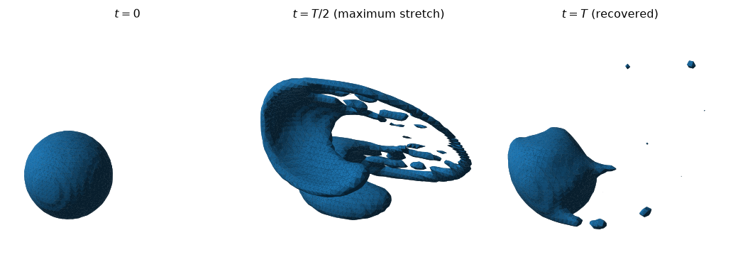
ns = np.array([32, 64, 128])
err = np.array([lv[n]["l1vol"] for n in ns])
fig, ax = plt.subplots(figsize=(4.9, 3.4))
ax.loglog(ns, err, "o-", color=BLUE, ms=7, lw=1.7, label="peclet (Weymouth–Yue + PLIC)")
ax.loglog(ns, err[0] * (ns / ns[0]) ** -2.0, "--", color="0.35", lw=1.2, label="second order")
for k, o in enumerate((ORDER1, ORDER)):
    ax.annotate(f"order {o:.2f}", xy=(np.sqrt(ns[k] * ns[k + 1]), np.sqrt(err[k] * err[k + 1])),
                xytext=(7, 3), textcoords="offset points", fontsize=9, color=BLUE)
ax.set(xlabel="grid resolution  (cells per unit box)",
       ylabel=r"$L_1$ shape error  (volume units)",
       title="LeVeque deformation, reversal at $T=3$")
ax.set_xticks(ns); ax.set_xticklabels([f"${n}^3$" for n in ns])
ax.minorticks_off(); ax.legend(fontsize=8); plt.show()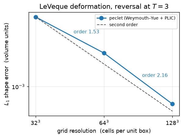
The headline: the shape error falls 7.75e-03 → 2.68e-03 → 5.98e-04, an order of 2.16 on the last interval. That is the published behaviour of a geometric PLIC scheme on this case — Cassinelli et al. report “asymptotically second-order convergence” for PLIC on exactly this test, with the coarse rung pre-asymptotic for the reason the middle panel of the figure makes obvious.
3. The conservation floor is the projection, not the grid
Now the number that separates a geometric VoF from an algebraic one. Look at the drift column of the table above: \(10^{-15}\), \(10^{-14}\), \(10^{-14}\) — over 800, 1600 and 3200 steps of a violently deforming flow, at three resolutions, with an error that does not scale with \(h\) in any recognisable way. It scales with the max|div| column sitting right next to it — to within a factor of two, at every resolution (Figure 5 collects every run on this page).
This is Equation 3, measured. The scheme’s volume error is \(\tfrac{\Delta t}{h}\sum_i c_i^{\,n}(\nabla\!\cdot\mathbf{u})_i\) accumulated over the run — so it is a property of the velocity field you hand it, not of the transport. In a coupled simulation that field comes from the pressure projection, which makes the statement operationally useful: the conservation error of a peclet two-phase run is the pressure solve’s divergence residual. Tighten the projection tolerance and the volume error goes down; refine the grid and it does not.
The failure mode: a velocity that is only analytically solenoidal
Which is why advect_vof refuses a field it does not believe. The natural way to use Equation 5 is to evaluate it at cell centres — that is how the paper states it — and hand those values over as face velocities. It is a perfectly convergent \(O(h)\) approximation of the right field and it is catastrophic here:
n = 32
ctr = (np.arange(n) + 0.5) / n
X, Y, Z = ctr[:, None, None], ctr[None, :, None], ctr[None, None, :]
one = np.ones((n, n, n))
uc = np.asfortranarray(2 * np.sin(PI*X)**2 * np.sin(2*PI*Y) * np.sin(2*PI*Z) * one * n)
vc = np.asfortranarray(-np.sin(2*PI*X) * np.sin(PI*Y)**2 * np.sin(2*PI*Z) * one * n)
wc = np.asfortranarray(-np.sin(2*PI*X) * np.sin(2*PI*Y) * np.sin(PI*Z)**2 * one * n)

def probe(geometry):
    s = flow.Solver(n, n, n)
    s.set_rho(1.0); s.set_mu(1.0); s.set_dt(3.75e-3)
    if geometry:                                     # all-fluid cut-cell operator
        s.set_pressure_geometry(np.full((n, n, n), 10.0, order="F"))
    s.enable_vof(); s.set_vof(sphere_fractions((n, n, n), .15*n, (.35*n,)*3))
    s.set_state(uc, vc, wc)
    return s

s = probe(geometry=True)
DIV_POINTWISE = s.max_open_divergence()
print(f"cell-centre sampled:  max|div(open u)| = {DIV_POINTWISE:.4f}")
try:
    s.advect_vof(3.75e-3); print("  advected (unexpected)")
except RuntimeError as e:
    print("  advect_vof refused:\n   ", str(e)[:186])
s.set_state(*leveque_fields(n))
print(f"discrete curl of @eq-potential:  max|div(open u)| = {s.max_open_divergence():.2e}"
      f"   ->   accepted")

# And what the guard is actually protecting you from, measured by disabling it:
s = probe(geometry=False)             # no cut-cell operator => max_open_divergence() is 0 by fiat
v0 = s.vof_diagnostics()["sum"]
for _ in range(50):
    s.advect_vof(3.75e-3)
LOSS = (s.vof_diagnostics()["sum"] - v0) / v0
print(f"\nsame field, guard inert (no pressure geometry): {100*LOSS:+.2f} % of the liquid "
      f"volume in 50 steps")
cell-centre sampled: max|div(open u)| = 0.6119
advect_vof refused:
advect_vof: the current face velocity is not discretely divergence-free (max|div(open*u)| = 0.61191 > 1e-10). Weymouth-Yue conservation is conditional on it; project the field first (ste
discrete curl of @eq-potential: max|div(open u)| = 7.11e-15 -> accepted
same field, guard inert (no pressure geometry): -4.93 % of the liquid volume in 50 stepsA divergence of 0.61 in cell units feeds Equation 3 directly: fifty steps of it destroy 4.9 % of the liquid volume — smoothly, with no NaN and with an interface that still looks entirely plausible. That second run had to be set up without a pressure geometry to happen at all — max_open_divergence() is an openness-weighted diagnostic and returns 0 by construction when the solver has no cut-cell operator, which switches the guard off with it. That is the one sharp edge on this API, and it is why every run on this page calls set_pressure_geometry even where there is no solid: an all-positive SDF costs nothing and keeps the guard live.
ImportantThe staggered sample is a special case, not a rule
Sampling Equation 5 pointwise on the staggered faces — \(u\) at \((i,\,j+\tfrac12,\,k+\tfrac12)\) and so on — happens to be discretely divergence-free too, exactly, by the identity \(\sin^2\pi x_{i+1}-\sin^2\pi x_i=\sin(2\pi x_{i+1/2})\sin(\pi h)\) applied to each of the three terms. That is a property of this field on this mesh, not a method. The vector-potential construction in Equation 6 is the method: it works for any prescribed field, on any staggered mesh, without a trigonometric identity having to come to the rescue.
The trap that is not visible in any bounded quantity
The freeze in Equation 2 is the single documented trap of this scheme. The dilation flag \(c^{\,n}_i = H(C^n_i-\tfrac12)\) must be computed once, from \(C^n\), and reused by all three sweeps; recomputing it between sweeps looks more accurate, changes nothing visible in the interface, and destroys the telescoping. WyAdvector::debugRecomputeDilation keeps that a measured number rather than folklore — 200 LeVeque steps at \(32^3\) give a drift of \(2.33\times10^{-15}\) frozen against \(1.455\times10^{-2}\) recomputed, a factor \(6\times10^{12}\). It is not exposed to Python, deliberately: it exists so the trap stays documented, not so it can be switched on.
4. How large a step a geometric scheme can take
Weymouth’s boundedness proof bounds the slab thickness at \(|a_f| = |u_f|\Delta t/h \le 1/(2(N-1))\) for \(N\)-dimensional flow — \(1/2\) in 2-D but \(1/4\) in 3-D. The widely quoted “CFL \(<0.5\)” is the 2-D value, and flow therefore ships the 3-D one as the default cap and throws above it:
s = flow.Solver(32, 32, 32)
s.set_rho(1.0); s.set_mu(1.0); s.set_dt(1.0)
s.set_pressure_geometry(np.full((32, 32, 32), 10.0, order="F"))
s.enable_vof(); s.set_vof(sphere_fractions((32, 32, 32), 8.0, (16., 16., 16.)))
s.set_state(*(np.asfortranarray(np.full((32, 32, 32), c)) for c in (1.0, 0.0, 0.0)))
print(f"default cap = {s.vof_cfl_limit()}   (Weymouth's 3-D bound 1/(2(N-1)))")
for dt in (0.25, 0.26):
    try:
        s.advect_vof(dt); print(f"  dt = {dt}: ran, interface Courant {s.vof_last_courant():.2f}")
    except RuntimeError as e:
        print(f"  dt = {dt}: refused — {str(e)[:96]}")
default cap = 0.25 (Weymouth's 3-D bound 1/(2(N-1)))
dt = 0.25: ran, interface Courant 0.25
dt = 0.26: refused — peclet::flow::vof::WyAdvector: CFL = max|uf| dt/h = 0.26 exceeds the Weymouth-Yue boundedness caThe cap is on the interface-local Courant number, not the global one: a quiescent far-field corner moving fast should not throttle a step that never touches the interface. vof_max_courant() reports it so you can size \(\Delta t\) directly (dt *= cfl_target / vof_max_courant()).
How tight is the bound? Not very — and it is worth knowing which way it fails. Re-run Zalesak with fewer, larger steps (the same one revolution, so the exact solution is unchanged) and watch conservation and boundedness come apart:
print(f"{'steps':>6} {'max CFL':>8} {'volume drift':>14} {'min C':>12} {'max C':>26} {'L1/V':>10}")
for steps, cap in ((1000, 0.5), (400, 1.0), (250, 1.5)):
    r = run_zalesak(steps=steps, cfl_cap=cap)
    print(f"{steps:>6} {r['cfl']:8.3f} {r['drift']:14.2e} {r['minC']:12.3e} "
          f"{r['maxC']:26.6g} {r['rel']:10.3e}")
steps max CFL volume drift min C max C L1/V
1000 0.311 0.00e+00 -3.778e-17 1 2.784e-02
400 0.778 0.00e+00 -4.629e-17 1 2.210e-02
250 1.244 -2.60e+39 -1.008e+58 9.28543e+57 5.024e+56At an interface Courant number of 0.78 — three times the shipped cap — the run is still exactly conservative and still bounded, and its shape error is even slightly lower (fewer steps, less reconstruction). Past \(|a_f|=1\) the geometric “flux” stops being a flux at all: the slab the sweep clips out is thicker than the donor cell, and the run detonates by fifty-odd orders of magnitude. The failure is on boundedness, in both directions — the bound is sufficient, not tight, and the quantity that tells you that you have crossed it is \(\min C\) / \(\max C\), never the volume.
NoteA wisp is not an interface, but the Courant band thinks it is
The interface-local band is “mixed cells and their face neighbours”, with neighbours compared by exact inequality. Weymouth–Yue leaves round-off colour residue behind it (\(\min C \approx -3\times10^{-17}\) above), and a cell holding \(10^{-17}\) differs from a neighbour holding \(0\) — so over a long run the band creeps outward along the interface’s wake. On the Zalesak run the reported interface Courant number starts at 0.254 and reaches 0.311, which is the global maximum: that is why this page raises the cap to 0.5 for a case whose interface never exceeds 0.255. The surface-tension path already guards its interfacial predicate with set_vof_interface_eps; the Courant band has no such guard yet.
5. Through an immersed solid
Everything above runs in an empty box. The same transport also runs through resolved geometry: with set_solid(sdf, cutcell_pressure=True), every geometric flux is weighted by the fluid area fraction \(o_f\) of its face, and the same \(o_f a_f\) enters the dilation term, so the telescoping in Equation 3 survives verbatim. The conserved functional becomes \(\sum_i \varepsilon^{\rm eff}_i C_i\) over the cells’ fluid volumes, with \(\varepsilon^{\rm eff} = \max(\varepsilon, 1/64)\) — the floor matters, because \(\varepsilon\) is built by \(4^3\) subsampling and a cell can read \(\varepsilon=0\) while still owning an open face. Such a cell is fluid, it receives flux, and the naive \(\sum\varepsilon C\) would silently drop whatever lands in it; vof_diagnostics() reports both (volume and raw_volume).
The test is the one the solver’s own gate battery uses: run the single-phase solver to a Stokes steady state through a periodic array of four spheres, freeze that projected velocity, and advect a liquid slab through it for 500 steps. Freezing the solver’s own output is the point — this is the field Equation 3 cares about, divergence residual and all.
def sphere_array_sdf(n, centres, radius):
    """Periodic sphere array; > 0 in fluid (flow's SDF sign), cell centres at i + 1/2."""
    a = [(np.arange(n) + .5).reshape([-1 if k == d else 1 for k in range(3)]) for d in range(3)]
    best = np.full((n, n, n), 1e30)
    for c in centres:
        for p in np.ndindex(3, 3, 3):
            sh = [(q - 1) * n for q in p]
            best = np.minimum(best, np.sqrt(sum((a[d] - (c[d] + sh[d]))**2
                                                for d in range(3))) - radius)
    return np.asfortranarray(best)

NPK = 48
f = NPK / 32.0
PACK = sphere_array_sdf(NPK, [(6*f, 7*f, 8*f), (20*f, 9*f, 23*f),
                              (11*f, 24*f, 19*f), (26*f, 22*f, 6*f)], 6.0 * f)

s = flow.Solver(NPK, NPK, NPK)
s.set_rho(1.0); s.set_mu(0.2); s.set_dt(1.0)
s.set_body_force(2e-3, 1e-3, 5e-4)
s.set_solid(PACK, cutcell_pressure=True)
iters = 0
for _ in range(60):
    s.step(); iters = max(iters, s.last_pressure_iterations())
DIV_PACK = s.max_open_divergence()

s.enable_vof()
C0_pack = np.zeros((NPK, NPK, NPK), order="F"); C0_pack[:, :, :NPK // 2] = 1.0
s.set_vof(C0_pack)
d0 = s.vof_diagnostics()
dt_pack = 0.2 / s.vof_max_courant()                 # interface Courant 0.2, CUT-CELL rule
clip, solid, mn, mx = 0.0, 0.0, 1e30, -1e30
for _ in range(500):
    s.advect_vof(dt_pack)
    d = s.vof_diagnostics()
    clip += d["clipped_volume"]; solid = max(solid, abs(d["solid_sum"]))
    mn, mx = min(mn, d["min_fluid"]), max(mx, d["max_fluid"])
d1, C_pack = s.vof_diagnostics(), s.get_vof()
DRIFT_PACK = (d1["volume"] - d0["volume"]) / d0["volume"]

print(f"{NPK}^3 packing: {d1['solid_cells']} solid cells, {d1['cut_cells']} cut cells;"
      f" Stokes converged in {iters} pressure iterations")
print(f"  projection residual   max|div(open u)| = {DIV_PACK:.3e}")
print(f"  500 kinematic steps at interface CFL 0.2 (dt = {dt_pack:.4g})")
print(f"  sum eps_eff*C   {d0['volume']:.15e} -> {d1['volume']:.15e}")
print(f"  relative drift  {DRIFT_PACK:.3e}      (floor: the projection residual above)")
print(f"  colour inside the solid          max|sum C| = {solid:.1e}   (exactly 0)")
print(f"  boundedness in UNCUT fluid cells  C in [{mn:.3g}, {mx:.17g}]")
print(f"  liquid volume moved by the clip over the whole run: {clip:.3e}")
48^3 packing: 9868 solid cells, 4612 cut cells; Stokes converged in 9 pressure iterations
projection residual max|div(open u)| = 3.920e-11
500 kinematic steps at interface CFL 0.2 (dt = 1.569)
sum eps_eff*C 4.876225000000000e+04 -> 4.876224999975420e+04
relative drift -5.041e-12 (floor: the projection residual above)
colour inside the solid max|sum C| = 0.0e+00 (exactly 0)
boundedness in UNCUT fluid cells C in [0, 1]
liquid volume moved by the clip over the whole run: 2.297e-18sl = 12 # a y-plane that cuts two of the four spheres
fig, axes = plt.subplots(1, 2, figsize=(7.0, 3.2))
for ax, (F, t) in zip(axes, [(C0_pack[:, sl, :], "initial slab"),
(C_pack[:, sl, :], "after 500 steps")]):
ax.imshow(np.where(PACK[:, sl, :] < 0, np.nan, F).T, origin="lower", cmap="Blues",
vmin=0, vmax=1, extent=(0, NPK, 0, NPK), interpolation="nearest")
ax.imshow(np.where(PACK[:, sl, :] < 0, 1.0, np.nan).T, origin="lower", cmap="Greys",
vmin=0, vmax=1.6, extent=(0, NPK, 0, NPK), interpolation="nearest")
ax.set(title=t, xlabel="x [cells]"); ax.grid(False)
axes[0].set_ylabel("z [cells]")
plt.tight_layout(); plt.show()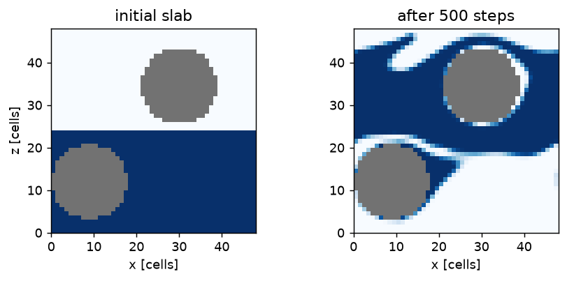
Drift -5.04e-12 against a projection residual of 3.92e-11 — the same statement as §3, now with the floor set by a real pressure solve instead of an analytic field. The clip that guards the cut-cell flux moved 2.3e-18 of liquid volume in 500 steps, i.e. it never fired; it is a tripwire on the flux approximation (the PLIC polyhedron is reconstructed on the whole cell and multiplied by the open area, rather than being clipped against the solid wall as well), not a mechanism.
WarningIn a cut cell the Courant limit is not the one you computed
The admissible slab thickness in a cell of fluid fraction \(\varepsilon_i\) behind a face of openness \(o_f\) is \(\max\!\big(|a_f|,\ o_f|a_f|/\max(\varepsilon_i,0.1)\big)\) — which reduces to \(|a_f|\) in clear fluid but is up to 6× tighter inside a packing. vof_max_courant() applies the cut-cell rule automatically when a solid is present, which is why the \(\Delta t\) above is computed from it rather than from \(\max|\mathbf{u}|\).
runs = [("Zalesak, 1000 steps", zal["div"], abs(zal["drift"]), BLUE, "o")]
for n in (32, 64, 128):
    runs.append((f"LeVeque ${n}^3$, {lv[n]['steps']} steps", lv[n]["div"], lv[n]["drift"],
                 GREEN, "s"))
runs.append((f"sphere packing ${NPK}^3$, 500 steps", DIV_PACK, abs(DRIFT_PACK), RED, "D"))
fig, ax = plt.subplots(figsize=(5.3, 3.8))
lim = (1e-17, 3e-10)
ax.plot(lim, lim, "-", color="0.6", lw=1.2, zorder=0)
ax.text(3e-14, 1.1e-14, "drift = divergence", color="0.45", fontsize=8, rotation=33)
for lbl, d, dr, col, mk in runs:
    ax.loglog(max(d, 1.5e-17), max(dr, 1.5e-17), mk, color=col, ms=8, label=lbl)
ax.axhspan(1e-17, 2.3e-16, color="0.92", zorder=0)
ax.text(2e-17, 1.1e-16, "double-precision round-off", fontsize=8, color="0.35")
ax.set(xlim=lim, ylim=lim,
       xlabel=r"divergence of the prescribed field  $\max|\nabla\!\cdot(o\,\mathbf{u})|$",
       ylabel="relative volume drift over the run",
       title="Where the conservation error comes from")
ax.legend(fontsize=8, loc="lower right"); plt.show()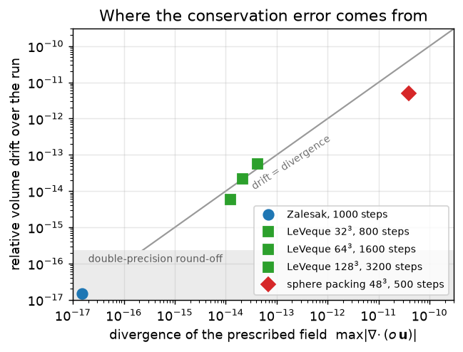
The point on the far right is the one that matters in practice: it is the only run on this page whose velocity came from a real pressure solve, and it keeps the same relationship to its own divergence residual as the analytic runs do — three decades further out along the same line. A geometric VoF has no conservation error of its own. It inherits the one upstream of it, which is a far easier thing to budget for than a truncation error.
Collocated cross-check
peclet also ships a cell-centred/collocated grid (flow.SolverColocated), and since rung V8 it carries the geometric VoF too. Its pressure coupling is an approximate (ABC) projection: the cell velocities are averaged onto a MAC face field, that field is projected exactly, and the correction is averaged back. The consequence for this page is the good kind of boring — the field the colour rides on, get_uf/get_vf/get_wf, is the one the projection makes discretely divergence-free, which is exactly the hypothesis Equation 3 needs, and it sits on the same faces: \(u_f(i)\) is the low \(x\)-face of cell \(i\), the same place the staggered \(u(i)\) lives. So the two grids do not run equivalent transport, they run the same kernel over the same array.
The check below makes that literal. The LeVeque case is run at \(32^3\) on the collocated grid — the analytic velocity (Equation 5) is uploaded at cell centres each step at the midpoint phase, and a step() with \(\mu=0\) and no forcing turns it into the projected face field, which then advects the colour. The identical uf/vf/wf is handed to a staggered Solver through set_state, advected with advect_vof(dt), and the two colour fields are differenced.
def leveque_cell(n):
    """@eq-leveque sampled at CELL CENTRES (the collocated unknown), in cell units."""
    c = (np.arange(n) + 0.5) / n
    X, Y, Z = c[:, None, None], c[None, :, None], c[None, None, :]
    u = 2 * np.sin(PI * X) ** 2 * np.sin(2 * PI * Y) * np.sin(2 * PI * Z)
    v = -np.sin(2 * PI * X) * np.sin(PI * Y) ** 2 * np.sin(2 * PI * Z)
    w = -np.sin(2 * PI * X) * np.sin(2 * PI * Y) * np.sin(PI * Z) ** 2
    return tuple(np.asfortranarray(np.broadcast_to(a, (n, n, n)).copy() * n)
                 for a in (u, v, w))

def leveque_colocated(n=32):
    steps = int(round(T_LV * 2 * n / CFL_LV))
    dt = T_LV / steps
    uc, vc, wc = leveque_cell(n)
    C0 = sphere_fractions((n, n, n), .15 * n, (.35 * n, .35 * n, .35 * n))
    sdf = np.full((n, n, n), 10.0, order="F")
    co = flow.SolverColocated(n, n, n)                 # the ABC grid: the run
    st = flow.Solver(n, n, n)                          # the mirror: same faces, same kernel
    for s in (co, st):
        s.set_rho(1.0); s.set_mu(0.0); s.set_dt(dt)
        s.set_pressure_geometry(sdf)
        s.enable_vof(); s.set_vof(C0)
    co.set_pressure_chebyshev(True, 500, 1e-14)
    d0, iters, div, dC = co.vof_diagnostics(), 0, 0.0, 0.0
    for i in range(steps):
        ph = np.cos(PI * (i + 0.5) * dt / T_LV)                  # the same midpoint phase
        co.set_state(*(np.asfortranarray(a * ph) for a in (uc, vc, wc)))
        co.step()                                                # projects -> uf/vf/wf, advects C
        iters = max(iters, co.last_pressure_iterations())
        div = max(div, co.max_open_divergence())
        st.set_state(co.get_uf(), co.get_vf(), co.get_wf())      # the SAME face field
        st.advect_vof(dt)
        if (i + 1) % 100 == 0 or i + 1 == steps:
            dC = max(dC, float(np.abs(co.get_vof() - st.get_vof()).max()))
    d1, C1 = co.vof_diagnostics(), co.get_vof()
    l1 = np.abs(C1 - C0).sum()
    return dict(n=n, steps=steps, l1vol=l1 / n**3, rel=l1 / C0.sum(), div=div, iters=iters,
                drift=(d1["sum"] - d0["sum"]) / d0["sum"], dC=dC, cap=500)

t0 = time.time()
col = leveque_colocated(32)
stg = lv[32]
print(f"LeVeque, T = 3 with reversal, 32^3, {col['steps']} steps   ({time.time()-t0:.0f} s)\n")
print(f"{'grid':>12} {'face field':>34} {'L1(vol)':>11} {'L1/V':>10} {'drift':>10} "
      f"{'max|div|':>10} {'pressure':>10}")
print(f"{'staggered':>12} {'discrete curl of @eq-potential':>34} {stg['l1vol']:11.4e} "
      f"{stg['rel']:10.4e} {stg['drift']:10.2e} {stg['div']:10.2e} {'n/a':>10}")
print(f"{'collocated':>12} {'ABC projection of the cell sample':>34} {col['l1vol']:11.4e} "
      f"{col['rel']:10.4e} {col['drift']:10.2e} {col['div']:10.2e} "
      f"{str(col['iters'])+'/'+str(col['cap']):>10}")
print(f"\nmax|C_colocated - C_staggered| over the run (same face field): {col['dC']:.3e}")
peclet::flow SolverColocated: AUTO scheme fell back to gauge-exact (geometric VoF on the collocated grid is rung V8 and the ghost projection v1 does not support it). Select explicitly with set_collocated_scheme to silence this notice.LeVeque, T = 3 with reversal, 32^3, 800 steps (44 s)
grid face field L1(vol) L1/V drift max|div| pressure
staggered discrete curl of @eq-potential 7.7465e-03 5.4794e-01 5.89e-15 1.24e-14 n/a
collocated ABC projection of the cell sample 7.7412e-03 5.4757e-01 -5.64e-15 1.07e-14 13/500
max|C_colocated - C_staggered| over the run (same face field): 0.000e+00The two colour fields differ by 0.0e+00 — not “to round-off”, bitwise, because after set_state the staggered solver’s advect_vof reads the identical doubles the collocated step() just advected with. The shape errors are not identical, and should not be: the collocated run’s face field is the projection of a cell-centred sample rather than the discrete curl, which differs from it by 0.24 % at \(32^3\), and the resulting L1/V differs by 0.07 %. The conservation floor is unmoved — -5.6e-15 against the staggered 5.9e-15 — because Equation 3 only ever asked for a discretely divergence-free face field, and an approximate projection delivers one on the faces exactly.
WarningOn the collocated grid,
advect_vof needs a step() first
set_state writes the cell velocity; the face field the colour rides on is built by the projection inside step(). Calling set_state and then advect_vof on a fresh SolverColocated therefore advects with a face field that is still all zeros — and the divergence guard does not catch it, because zero is divergence-free. Seed the face field with a step() (as above) before advecting kinematically. On the staggered grid set_state writes the faces directly, so the pattern in §1 and §2 is fine there.
Adapt this yourself
- Bring your own velocity. Anything you can put on the staggered faces with
set_stateand that survives the divergence guard is a valid transport test — a shear layer, a vortex pair, a measured PIV field. If yours does not survive the guard, build it as a discrete curl the way Equation 6 does; it is almost always easier than fixing the sampled field afterwards. - Use the solver’s own field instead. Run
step()to a steady state, thenadvect_vof(dt)in a loop, exactly as §5 does. This is the cheapest way to study transport through a geometry you care about without paying for the momentum solve every step. - Push the reversal time. \(T=3\) is the standard; \(T=6\) or \(T=8\) leaves the interface under-resolved for twice as long and is where PLIC’s first-order corner error is easiest to see. The volume drift will not move.
- Turn on the physics. Everything here is kinematic.
set_property_modelfor \(\rho(C)\) and \(\mu(C)\),set_surface_tension, andstep()in place ofadvect_vofturns this into a coupled two-phase run — see Parasitic currents and Rising bubble. - Go multi-rank. The same script runs under
mpirun -np N python …; the colour field carries its own \(g=3\) halo and the advection is bitwise decomposition-independent at np = 1, 2, 4.
Reproduce this
The compiled solver runs this, so its outputs are frozen into the site. To regenerate:
pip install peclet            # the solver, from PyPI
quarto render examples/vof-advection-benchmarks/index.qmd --execute
# ...or against a local source build of the suite (GPU):
PECLET_LOCAL_BUILD=/path/to/suite/flow/build_cuda OMP_NUM_THREADS=8 OMP_PROC_BIND=false \
  quarto render examples/vof-advection-benchmarks/index.qmd --execute
The same battery lives inside the solver repo as the vof_advect ctest (tests/kokkos/test_vof_advect.cpp, with the scene builders in tests/kokkos/vof_advect_scenes.hpp) and, for §5, as tests/study/vof_cutcell.py g2; the MPI siblings (vof_advect_mpi_np{1,2,4}) gate the bitwise decomposition-independence.
One number to square: the in-repo vof_advect ctest reports \(2.81\times10^{-2}\) for the Zalesak case against the \(2.78\times10^{-2}\) above. Its scene builder samples the \(y\)-face velocity half a cell off the face centre, so its flow is a rigid rotation about a point \(h/2\) away from ours — and a full revolution is the identity map about any centre, which is why the two shape errors agree to 1 % rather than differing structurally.
References
Aulisa, E., S. Manservisi, R. Scardovelli, and S. Zaleski. 2007. “Interface Reconstruction with Least-Squares Fit and Split Advection in Three-Dimensional Cartesian Geometry.” Journal of Computational Physics 225 (2): 2301–19. https://doi.org/10.1016/j.jcp.2007.03.015.
LeVeque, Randall J. 1996. “High-Resolution Conservative Algorithms for Advection in Incompressible Flow.” SIAM Journal on Numerical Analysis 33 (2): 627–65. https://doi.org/10.1137/0733033.
Weymouth, G. D., and Dick K.-P. Yue. 2010. “Conservative Volume-of-Fluid Method for Free-Surface Simulations on Cartesian-Grids.” Journal of Computational Physics 229 (8): 2853–65. https://doi.org/10.1016/j.jcp.2009.12.018.
Zalesak, Steven T. 1979. “Fully Multidimensional Flux-Corrected Transport Algorithms for Fluids.” Journal of Computational Physics 31 (3): 335–62. https://doi.org/10.1016/0021-9991(79)90051-2.