import importlib.util, os, subprocess, sys
# dem's step is deterministic only single-threaded; set this BEFORE the module is imported,
# because Kokkos reads it at initialisation. The POUR below is multithreaded on purpose (a pack
# is not a determinism claim) — see the note in "Pour it".
os.environ.setdefault("OMP_NUM_THREADS", "8")
os.environ.setdefault("OMP_PROC_BIND", "false")
_local = os.environ.get("PECLET_LOCAL_BUILD")
if _local:
for p in _local.split(os.pathsep):
sys.path.insert(0, p)
elif importlib.util.find_spec("peclet") is None:
subprocess.run([sys.executable, "-m", "pip", "install", "-q", "peclet", "scikit-image"],
check=True)Pall rings: packing a composed analytic particle
Author an industrial packing element as a CSG tree — a certified hollow cylinder minus its windows, plus two webs — measure it by implicit quadrature, and pour fifty of them into a periodic box with peclet.dem.
dem
sdf
csg
packing
granular
porous
 About six minutes on a CPU — most of it the pour.
What you’ll learn
A Pall ring is a hollow cylinder with windows punched through the wall and the punched-out tongues bent inward. It is the workhorse random packing of absorption and distillation columns, and it is also a good stress test for a particle representation: it is concave, thin-walled, and its whole point is that fluid threads through it.
This page builds one as a CSG tree in peclet.core.geom and packs fifty of them. Along the way:
- A CSG design decision with a measurable payoff.
difference(A, B)inherits the left child’s bounding-ball certificate, so building the ring asdifference(hollow_cylinder, windows)keeps a certificate thatdifference(hollow_cylinder_shell, windows)throws away. We check both, and the difference is stark: 0% versus 24.7% of exterior probes violating the bound the scene query prunes on. - Mass properties of a shape with no closed form, by implicit quadrature — volume, centre of mass, principal moments and the quaternion that reaches them.
- The pack, and the honest reading of its porosity: our ring is a thick-walled mini, and comparing its bed voidage with a table of real 1-inch Pall rings would be meaningless. What transfers is the envelope packing fraction, and we use it to show the whole gap is wall thickness.
The frozen pack is committed as a small .npz, and is the input to the companion page that pushes flow through it.
NoteRequires a recent
peclet
The CSG authoring layer (peclet.core.geom), composed analytic particles (Simulation.add_scene_shape) and the peclet.dem.scene_particle one-call pipeline are newer than the current PyPI release; on Colab you need a source build of peclet-core and peclet-dem until the next release goes out. The page is frozen, so it renders and reads correctly either way.
import time
import numpy as np
import matplotlib.pyplot as plt
from matplotlib import animation
from mpl_toolkits.mplot3d.art3d import Poly3DCollection
from scipy.spatial import cKDTree
from skimage import measure
from peclet.core import geom
from peclet import dem as pdem
from peclet.dem import scene_particle
plt.rcParams.update({"figure.dpi": 130, "font.size": 9, "axes.axisbelow": True,
"figure.facecolor": "white", "savefig.bbox": "tight"})
T_PAGE = time.time()Step 1 — The ring, and why the CSG order matters
Everything is in units of the ring’s outer diameter \(D = 2R_o = 1\). Height equals diameter, as it does for a real Pall ring.
R_O, H, T = 0.5, 1.0, 0.12 # outer radius, height, wall thickness
R_I = R_O - T
NWIN, YWIN = 4, 0.24 # windows per row; the two rows sit at y = ±YWIN
WR, WA, WT = 0.16, 0.17, 0.13 # window box half-extents: radial, axial, tangential
WEB = (0.40, 0.06, 0.06) # inner web plate half-extents
def qy(a):
"""Quaternion (x,y,z,w) for a rotation by `a` about the y axis."""
return [0.0, float(np.sin(0.5 * a)), 0.0, float(np.cos(0.5 * a))]
def pall_ring(b, certified=True):
# The tube. core's `hollow_cylinder` [rOuter, height, thickness] is about y and is
# DISTANCE-EXACT; `hollow_cylinder_shell` describes the same solid but is only SIGN-exact.
if certified:
tube = b.add_leaf("hollow_cylinder", [R_O, H, T])
else:
tube = b.add_leaf("hollow_cylinder_shell", [R_O, R_I, H],
rotation=[float(np.sin(np.pi / 4)), 0.0, 0.0, float(np.cos(np.pi / 4))])
# Two rows of window boxes, the lower row rotated half a pitch, each box's local x pointing
# radially outward and spanning the whole wall.
wins = []
for row, ysign in enumerate((+1, -1)):
for k in range(NWIN):
phi = 2 * np.pi * k / NWIN + (np.pi / NWIN if row else 0.0)
wins.append(b.add_leaf("box", [WR, WA, WT],
translation=[R_O * np.cos(phi), ysign * YWIN,
R_O * np.sin(phi)],
rotation=qy(-phi)))
w = wins[0]
for x in wins[1:]:
w = b.add_union(w, x)
# THE DESIGN DECISION: tube on the LEFT of the difference.
shell = b.add_difference(tube, w)
# ...and the two inner webs, unioned on (union keeps the certificate iff BOTH children have it,
# and a box leaf does).
return b.add_union(
b.add_union(shell, b.add_leaf("box", list(WEB), translation=[0.0, +YWIN, 0.0])),
b.add_leaf("box", list(WEB), translation=[0.0, -YWIN, 0.0], rotation=qy(np.pi / 2)))
b = geom.SceneBuilder()
ring = pall_ring(b, certified=True)
b_bad = geom.SceneBuilder()
ring_bad = pall_ring(b_bad, certified=False)
print("nodes in the tree: %d" % b.num_nodes())nodes in the tree: 21Step 2 — The certificate, tested
peclet.core’s scene query prunes candidate primitives with a bounding-ball bound. The bound is valid only when the field satisfies
\[ \varphi(\mathbf p) \;\ge\; \operatorname{dist}\!\big(\mathbf p,\; B\big), \qquad B = \text{a ball containing the solid}, \tag{1}\]
for every exterior point. That holds for exact-distance leaves and is preserved by union (when both children have it) and by intersection and difference (which keep the left child’s ball, since \(\max(a,\cdot)\ge a\)). It fails for the under-estimating leaves — ellipsoid, superquadric, hollow_cylinder_shell — and an instance without a certificate is never pruned: it rides an always list and is evaluated for every single query.
So the two trees above describe the same solid and cost very differently. Let’s check both claims.
# The root ball that nodeBound() derives: hollow_cylinder gives a ball at the origin of radius
# sqrt(rOuter^2 + (height/2)^2), and the union with the webs keeps it iff the web balls fit inside.
R_BALL = np.sqrt(R_O ** 2 + (H / 2) ** 2)
assert YWIN + np.linalg.norm(WEB) <= R_BALL, "web ball escapes the tube's ball"
rng = np.random.default_rng(11)
# 1) the two trees must describe the SAME solid
q = rng.uniform(-1.0, 1.0, size=(200_000, 3))
same = (np.sign(np.asarray(b.eval_root(ring, q)))
== np.sign(np.asarray(b_bad.eval_root(ring_bad, q)))).mean()
# 2) probe strictly outside the ball and compare phi against the distance to the ball
u = rng.normal(size=(200_000, 3)); u /= np.linalg.norm(u, axis=1)[:, None]
r = R_BALL * (1.0 + rng.random(200_000) * 1.4)
p = u * r[:, None]
lower = r - R_BALL
cert_rows = []
for lbl, bb, rr in (("certified (hollow_cylinder)", b, ring),
("uncertified (hollow_cylinder_shell)", b_bad, ring_bad)):
phi = np.asarray(bb.eval_root(rr, p))
slack = phi - lower
viol = slack < 0
cert_rows.append((lbl, slack.min(), 100 * viol.mean(),
(phi[viol] / lower[viol]).min() if viol.any() else 1.0))
print("root bounding ball: centre origin, radius %.6f" % R_BALL)
print("the two trees agree in SIGN on %.4f%% of 200k points\n" % (100 * same))
print("%-36s min(phi - dist_to_ball) violating worst ratio" % "")
for lbl, mn, pc, wr in cert_rows:
print("%-36s %+.6f %6.2f%% %.4f" % (lbl, mn, pc, wr))root bounding ball: centre origin, radius 0.707107
the two trees agree in SIGN on 100.0000% of 200k points
min(phi - dist_to_ball) violating worst ratio
certified (hollow_cylinder) +0.000000 0.00% 1.0000
uncertified (hollow_cylinder_shell) -0.288011 24.68% 0.7071Same solid, and the certified construction satisfies Equation 1 with zero violations while the sign-exact one breaks it on a quarter of the exterior — worst case \(\varphi/\!\operatorname{dist}
= 1/\sqrt2\), the corner under-run you get from a max of half-space distances. Ordering the difference the other way round would have cost the same certificate.
Step 3 — Measure it, reframe it, shell it
t0 = time.time()
sp = scene_particle.build(b, ring, bounds=([-0.56] * 3, [0.56] * 3), n=32,
shell_resolution=112, target_shell_points=1200)
V_ENV = np.pi * R_O ** 2 * H # the cylinder the ring is inscribed in
print("scene_particle.build: %.1f s" % (time.time() - t0))
print("solid volume %.6f (%.4f of the envelope cylinder %.4f)"
% (sp.volume, sp.volume / V_ENV, V_ENV))
print("centre of mass %s" % np.round(sp.com, 6))
print("principal moments %s" % np.round(sp.principal, 7))
print("bounding radius %.4f shell probes %d" % (sp.bounding_radius, len(sp.shell)))scene_particle.build: 19.6 s
solid volume 0.268032 (0.3413 of the envelope cylinder 0.7854)
centre of mass [2.00e-06 6.67e-04 2.00e-06]
principal moments [0.0480566 0.0481478 0.0498186]
bounding radius 0.7191 shell probes 1211peclet.dem collides against the exact tree; the shell is only a set of surface probe points, and their spacing is what bounds contact resolution. The rule of thumb is probe spacing \(\lesssim\) (smallest feature)/3, and the smallest feature here is the wall — so let’s measure the spacing rather than assume it.
d_nn, _ = cKDTree(sp.shell).query(sp.shell, k=2)
MIN_FEATURE = min(T, 2 * WEB[1])
print("probe nearest-neighbour spacing: median %.4f mean %.4f p90 %.4f"
% (np.median(d_nn[:, 1]), d_nn[:, 1].mean(), np.percentile(d_nn[:, 1], 90)))
print("smallest feature %.3f -> target spacing <= %.4f %s"
% (MIN_FEATURE, MIN_FEATURE / 3,
"MET" if np.median(d_nn[:, 1]) <= MIN_FEATURE / 3 else "NOT MET"))probe nearest-neighbour spacing: median 0.0369 mean 0.0383 p90 0.0596
smallest feature 0.120 -> target spacing <= 0.0400 METCode
HALF, NB = 0.62, 150
SPC = 2 * HALF / (NB - 1)
gv = np.asarray(b.bake(sp.home_root, origin=[-HALF] * 3, spacing=[SPC] * 3, dims=[NB] * 3))
V3, F3_, _, _ = measure.marching_cubes(
np.ascontiguousarray(gv.reshape(NB, NB, NB, order="F")), level=0.0, spacing=(SPC,) * 3)
V3 = V3 - HALF
AREA = measure.mesh_surface_area(V3, F3_)
fig = plt.figure(figsize=(5.4, 3.0))
for k, (elev, azim, ttl) in enumerate([(22, 35, "outside"), (78, 20, "down the bore")]):
ax = fig.add_subplot(1, 2, k + 1, projection="3d")
ax.add_collection3d(Poly3DCollection(V3[F3_], facecolor="#8ea9c4", edgecolor="none"))
ax.set_xlim(-0.6, 0.6); ax.set_ylim(-0.6, 0.6); ax.set_zlim(-0.6, 0.6)
ax.set_box_aspect((1, 1, 1)); ax.set_axis_off(); ax.view_init(elev=elev, azim=azim)
ax.set_title(ttl, fontsize=8)
plt.show()
print("surface area %.4f D^2 specific surface A/V_envelope = %.3f / D" % (AREA, AREA / V_ENV))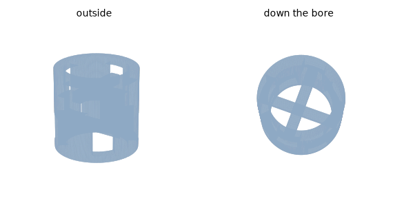
surface area 6.5607 D^2 specific surface A/V_envelope = 8.353 / DStep 4 — Pour it
Fifty rings dropped into a box that is periodic in \(x\) and \(z\) (so there are no column walls at all) onto an analytic floor, then tapped twice and quenched.
ImportantA
peclet.dem trap, and a bug this page found and got fixed
set_positions resets every particle to shape 0, so set_shape_ids must come after it — that one is permanent, and it is in the docstring.
The second was a real defect. Writing this page, composed-tree grains fell straight through the floor, and at 48 rings × 1625 shell probes the run corrupted the heap and aborted around step 2000. Both were the same cause: every contact buffer was sized from the particle capacity at the moment a shape was registered, while demStep grows that capacity on every step (it adds ghost headroom), so the buffers were left behind and the narrow phase’s boundary contacts — appended after the body-body ones — fell off the end. add_scene_shape also never called the sizing routine at all, which every sibling adder does. Fixed in peclet.dem (growContactBuffers now runs wherever the capacity grows), with a regression that drops composed-tree grains onto a plane from a deliberately small construction capacity. The workaround this page originally carried — constructing the Simulation far larger than the particle count — is no longer needed. See ISSUES.md.
L, N, DT = 3.5, 48, 2e-3 # box side (in ring diameters), ring count, time step
rng = np.random.default_rng(5)
pos, y = [], 1.2
while len(pos) < N: # a loose non-overlapping cloud to drop from
c = np.array([rng.uniform(0, L), y, rng.uniform(0, L)])
if all(np.linalg.norm((c - q)[[0, 2]]) > 1.55 or abs(c[1] - q[1]) > 1.55 for q in pos[-14:]):
pos.append(c)
else:
y += 0.15
pos = np.asarray(pos, dtype=np.float32)
quat0 = rng.normal(size=(N, 4)); quat0 /= np.linalg.norm(quat0, axis=1)[:, None]
sim = pdem.Simulation(N + 8) # the buffers now follow the capacity; no headroom needed
sim.set_domain((0.0, -1.2, 0.0), (L, 60.0, L))
sim.enable_periodicity(True, False, True)
sim.set_gravity(0.0, -9.81, 0.0)
sim.set_material_params(0.15, 0.0, 0.5) # restitution_n, restitution_t, friction
sim.set_solver_iterations(10, 8)
shape_id = sp.register(sim)
# The floor is an ANALYTIC WALL — a solid box below y = 0, so the container is a CSG tree too.
fb = geom.SceneBuilder()
floor = fb.add_leaf("box", [40.0, 1.0, 40.0], translation=[L / 2, -1.0, L / 2])
fi, fr, _, _ = fb.encode()
sim.add_analytic_wall(np.asarray(fi, np.int32), np.asarray(fr, np.float32),
floor, False, 0.15, 0.5)
sim.set_positions(pos)
sim.set_shape_ids(np.full(N, shape_id, np.int32)) # AFTER set_positions
sim.set_quaternions(quat0.astype(np.float32))
sim.set_inv_mass(np.full(N, 1.0 / sp.mass, np.float32))
sim.set_inv_inertia(np.tile(sp.inv_inertia_unit, (N, 1)).astype(np.float32))
sim.set_dt(DT)The protocol is pour → tap → quench. The taps shake the bed off whatever loose arrangement it first fell into; the quench (damping the velocities by 4% per step) removes the residual jitter, so what we freeze is a static pack rather than a snapshot of a bed still rattling.
frames, ke_hist, t_hist = [], [], []
step_no = [0]
def kinetic():
v = np.asarray(sim.get_velocities()); w = np.asarray(sim.get_angular_velocities())
return float(0.5 * sp.mass * (v ** 2).sum() + 0.5 * (np.asarray(sp.principal) * w ** 2).sum())
def advance(n, damp=None, every=45):
for i in range(n):
sim.step(DT) # step() with NO argument advances nothing
if damp is not None:
sim.set_velocities((np.asarray(sim.get_velocities()) * damp).astype(np.float32))
sim.set_angular_velocities(
(np.asarray(sim.get_angular_velocities()) * damp).astype(np.float32))
step_no[0] += 1
if i % every == 0:
frames.append((np.asarray(sim.get_positions()).copy(),
np.asarray(sim.get_quaternions()).copy()))
ke_hist.append(kinetic()); t_hist.append(step_no[0] * DT)
t0 = time.time()
advance(1400) # pour
for _ in range(2): # two taps
v = np.asarray(sim.get_velocities()).copy(); v[:, 1] += 0.8
sim.set_velocities(v.astype(np.float32))
advance(400)
advance(600) # relax
advance(900, damp=0.96) # quench
T_POUR = time.time() - t0
P = np.asarray(sim.get_positions()).astype(float)
Q = np.asarray(sim.get_quaternions()).astype(float); Q /= np.linalg.norm(Q, axis=1)[:, None]
KE_END = kinetic()
E_SCALE = N * sp.mass * 9.81 * (2 * R_O) # lifting the whole bed one diameter
MAXOV = sim.compute_overlaps()
print("%d steps in %.0f s (%.0f ms/step)" % (step_no[0], T_POUR, 1e3 * T_POUR / step_no[0]))
print("bed occupies y = %.2f .. %.2f (box %.1f x %.1f ring diameters)" % (P[:,1].min(), P[:,1].max(), L, L))
print("residual kinetic energy %.3e = %.2e of a one-diameter lift of the whole bed"
% (KE_END, KE_END / E_SCALE))
print("max contact overlap %.4f = %.0f%% of the wall thickness" % (MAXOV, 100 * MAXOV / T))3700 steps in 299 s (81 ms/step)
bed occupies y = 0.50 .. 5.53 (box 3.5 x 3.5 ring diameters)
residual kinetic energy 5.950e-02 = 4.71e-04 of a one-diameter lift of the whole bed
max contact overlap 0.0272 = 23% of the wall thicknessCode
fig, ax = plt.subplots(figsize=(6.0, 2.4))
ax.semilogy(t_hist, np.maximum(ke_hist, 1e-6), color="#4c72b0", lw=1.1)
for lbl, s_ in (("pour", 0), ("tap", 1400), ("tap", 1800), ("relax", 2200), ("quench", 2800)):
ax.axvline(s_ * DT, color="0.8", lw=0.7, zorder=0)
ax.text(s_ * DT + 0.05, 0.8 * max(ke_hist), lbl, fontsize=7, color="0.4")
ax.set_xlabel("time"); ax.set_ylabel("kinetic energy"); ax.grid(alpha=0.3)
plt.show()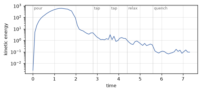
NoteWhat is and is not deterministic here
The pour runs multithreaded: peclet.dem’s step is bitwise reproducible only at OMP_NUM_THREADS=1, and a random pack is not a determinism claim, so there is nothing to gain from serialising it. Everything downstream — the certificate test, the mass properties, and all the pack statistics — is computed from the frozen state with deterministic host code, so it is reproducible from the committed .npz regardless of how the pour was run.
Code
NFR = 60
sel = np.linspace(0, len(frames) - 1, NFR).astype(int)
probe = sp.shell[::max(1, len(sp.shell) // 90)]
colr = plt.cm.viridis(plt.Normalize()(pos[:, 1]))
def qmat(q):
x, y_, z, w = q
return np.array([[1-2*(y_*y_+z*z), 2*(x*y_-z*w), 2*(x*z+y_*w)],
[2*(x*y_+z*w), 1-2*(x*x+z*z), 2*(y_*z-x*w)],
[2*(x*z-y_*w), 2*(y_*z+x*w), 1-2*(x*x+y_*y_)]])
figm = plt.figure(figsize=(3.4, 4.0)); axm = figm.add_subplot(111, projection="3d")
def draw(k):
axm.clear()
Pk, Qk = frames[sel[k]]
for i in range(N):
w = Pk[i] + probe @ qmat(Qk[i] / np.linalg.norm(Qk[i])).T
axm.scatter(w[:, 0], w[:, 2], w[:, 1], s=0.8, color=colr[i], depthshade=False)
axm.set_xlim(0, L); axm.set_ylim(0, L); axm.set_zlim(0, 8)
axm.set_box_aspect((1, 1, 2.3)); axm.set_axis_off(); axm.view_init(elev=14, azim=-62)
axm.set_title("t = %5.2f" % t_hist[sel[k]], fontsize=8)
return []
anim = animation.FuncAnimation(figm, draw, frames=NFR, interval=70, blit=False)
plt.close(figm)
from IPython.display import HTML
HTML(anim.to_jshtml(fps=14))Step 5 — What the pack looks like, numerically
Porosity is measured by Monte Carlo directly on the analytic trees — no voxelisation — over a bulk window that excludes the floor layer and the free surface, with the periodic images in \(x\) and \(z\) included.
R = np.array([qmat(q) for q in Q])
shift = np.array([[i * L, 0, j * L] for i in (-1, 0, 1) for j in (-1, 0, 1)])
Pe = (P[None, :, :] + shift[:, None, :]).reshape(-1, 3)
Re = np.tile(R, (9, 1, 1)); owner = np.tile(np.arange(N), 9)
tree = cKDTree(Pe); BR = float(sp.bounding_radius)
def fractions(y0, y1, K=400_000, seed=0):
g = np.random.default_rng(seed)
S = np.column_stack([g.uniform(0, L, K), g.uniform(y0, y1, K), g.uniform(0, L, K)])
cand = tree.query_ball_point(S, BR)
pi = np.concatenate([np.full(len(c), k) for k, c in enumerate(cand) if c])
ri = np.concatenate([np.asarray(c) for c in cand if c])
loc = np.einsum('nij,nj->ni', np.transpose(Re[ri], (0, 2, 1)), S[pi] - Pe[ri])
phi = np.asarray(b.eval_root(sp.home_root, np.ascontiguousarray(loc)))
solid = np.zeros(K, bool); np.logical_or.at(solid, pi, phi < 0.0)
nin = np.zeros(K, int); np.add.at(nin, pi, (phi < 0.0).astype(int))
env = np.zeros(K, bool)
np.logical_or.at(env, pi, (np.hypot(loc[:, 0], loc[:, 2]) <= R_O) & (np.abs(loc[:, 1]) <= H / 2))
return 1.0 - solid.mean(), env.mean(), (nin >= 2).mean()
YTOP = P[:, 1].max()
windows = [(1.00, YTOP - 0.80), (0.80, YTOP - 0.60), (1.20, YTOP - 1.00)]
res = [fractions(*w) for w in windows]
EPS, F_ENV, OVLAP = res[0]
print(" bulk window porosity eps envelope fraction f_env doubly-covered volume")
for (y0, y1), (e, f, o) in zip(windows, res):
print(" y = %.2f .. %.2f %.4f %.4f %.5f" % (y0, y1, e, f, o))
print("\nspread over the three windows: eps %.4f +/- %.4f"
% (np.mean([r[0] for r in res]), np.std([r[0] for r in res]))) bulk window porosity eps envelope fraction f_env doubly-covered volume
y = 1.00 .. 4.73 0.7998 0.5818 0.00009
y = 0.80 .. 4.93 0.7973 0.5751 0.00013
y = 1.20 .. 4.53 0.7976 0.5867 0.00012
spread over the three windows: eps 0.7982 +/- 0.0011# Coordination. A pair touches if either ring has a probe inside the other's tree — the test has
# to be run BOTH ways, because for interlocking concave bodies it is not symmetric: a rim can
# thread a window so that one ring's probes miss while the other's do not.
def probes_inside(a_pos, a_rot, b_pos, b_rot):
loc = ((a_pos + sp.shell @ a_rot.T) - b_pos) @ b_rot
return np.asarray(b.eval_root(sp.home_root, np.ascontiguousarray(loc))).min() < 0.0
cnt = np.zeros(N, int); npair = 0
for i in range(N):
for j in tree.query_ball_point(P[i], 2 * BR):
if owner[j] == i:
continue
npair += 1
if (probes_inside(P[i], R[i], Pe[j], Re[j])
or probes_inside(Pe[j], Re[j], P[i], R[i])):
cnt[i] += 1
Z_MEAN = cnt.mean(); RATTLERS = int((cnt < 1).sum())
# Orientation: the ring axis is +y in the frame we authored, so in the principal body frame it is
# R(quat)^T e_y — computed once, then carried into the world frame by each particle's quaternion.
AX_BODY = qmat(np.asarray(sp.quat, float)).T @ np.array([0.0, 1.0, 0.0])
cos_v = np.abs(np.einsum('nij,j->ni', R, AX_BODY)[:, 1])
SEM = (1 / np.sqrt(12)) / np.sqrt(N) # s.e.m. of |cos| for a uniform (isotropic) axis
print("mean coordination number %.2f rattlers (no contact) %d candidate pairs %d (ordered)"
% (Z_MEAN, RATTLERS, npair))
print("ring-axis |cos(theta from vertical)|: mean %.4f +/- %.4f (s.e.m.) -- isotropic is 0.500"
% (cos_v.mean(), SEM))mean coordination number 3.75 rattlers (no contact) 0 candidate pairs 396 (ordered)
ring-axis |cos(theta from vertical)|: mean 0.5265 +/- 0.0417 (s.e.m.) -- isotropic is 0.500Code
NBB = 46
SPB = 2 * HALF / (NBB - 1)
gb = np.asarray(b.bake(sp.home_root, origin=[-HALF] * 3, spacing=[SPB] * 3, dims=[NBB] * 3))
Vb, Fb, _, _ = measure.marching_cubes(
np.ascontiguousarray(gb.reshape(NBB, NBB, NBB, order="F")), level=0.0, spacing=(SPB,) * 3)
Vb = Vb - HALF
fig = plt.figure(figsize=(7.0, 3.4))
ax = fig.add_subplot(1, 2, 1, projection="3d")
cb = plt.cm.viridis(plt.Normalize(P[:, 1].min(), P[:, 1].max())(P[:, 1]))
for i in range(N):
ax.add_collection3d(Poly3DCollection(((Vb @ R[i].T) + P[i])[Fb][:, :, [0, 2, 1]],
facecolor=cb[i], edgecolor="none"))
ax.set_xlim(0, L); ax.set_ylim(0, L); ax.set_zlim(0, P[:, 1].max() + 0.6)
ax.set_box_aspect((1, 1, 1.5)); ax.set_axis_off(); ax.view_init(elev=16, azim=-62)
ax2 = fig.add_subplot(1, 2, 2)
ax2.hist(cos_v, bins=np.linspace(0, 1, 9), density=True, color="#8ea9c4", edgecolor="w")
ax2.axhline(1.0, color="#c44e52", lw=1.4, label="isotropic")
ax2.set_xlabel(r"$|\cos\theta|$ of the ring axis from vertical"); ax2.set_ylabel("density")
ax2.legend(fontsize=8, frameon=False); ax2.grid(alpha=0.3)
plt.show()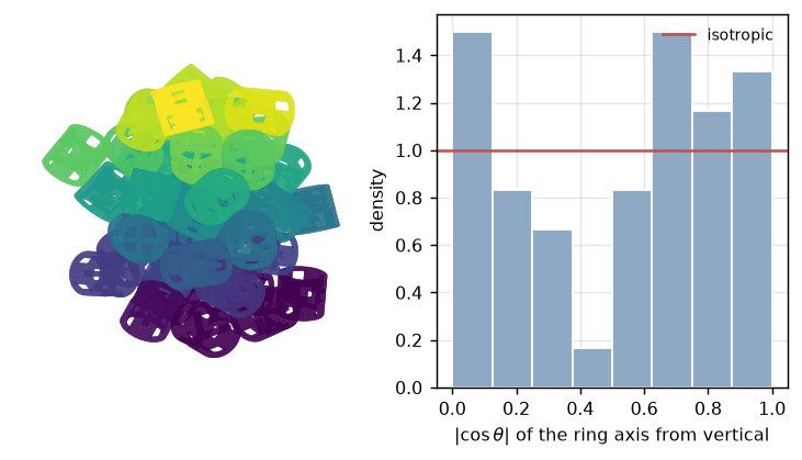
Each ring touches 3.75 others on average, counting a contact only where one ring’s probes are strictly inside the other’s tree. That sits at about the isostatic bound — roughly 4 contacts per body for a frictional packing of rigid non-spherical shapes, where friction supplies the tangential constraints — so the bed is marginally rigid rather than comfortably jammed. Together with the residual jitter above, the honest description is a loose bed held partly by interlocking. A denser pack would need a harder protocol (more taps, a longer quench, or compaction under a lid) and would give a lower \(\varepsilon\).
The ring axes come out at \(\lvert\cos\theta\rvert =\) 0.526 ± 0.042 against the isotropic 0.500 — a hint that the rings prefer to lie with their axes off-vertical, as dumped short cylinders do, but at 0.6 standard errors on 48 rings it is not a result. Resolving it would need a few hundred rings, and that is a different page.
Step 6 — Porosity, honestly
Our bed voidage is \(\varepsilon =\) 0.800. Published tables for real 25 mm Pall rings give roughly \(\varepsilon \approx 0.90\)–\(0.95\) for thin-walled metal and plastic rings, and \(\approx 0.74\)–\(0.78\) for ceramic ones, whose walls are proportionally much thicker (Billet and Schultes 1999; Stichlmair et al. 1989). Quoting a percentage agreement against either would be meaningless: our ring’s wall is \(t/D =\) 0.12, several times thicker than a metal Pall ring’s sheet. It is a thick-walled mini, and the comparison below is to the published range and its mechanism, not to a tabulated row.
What does transfer is how densely the rings’ cylindrical envelopes pack, because that is a property of the shape’s outline and the deposition, not of its wall:
\[ \varepsilon \;=\; 1 - f_{\text{env}}\, s , \qquad f_{\text{env}} = \frac{N V_{\text{env}}}{V_{\text{bed}}}, \qquad s = \frac{V_{\text{solid}}}{V_{\text{env}}} . \tag{2}\]
We measure \(f_{\text{env}} =\) 0.582 — comfortably below the \(\approx 0.64\) of random close-packed spheres and below the \(0.629\) this gallery’s own random packed bed measured with peclet.dem, which is what you expect for frictional, non-spherical, gravity-deposited bodies.
Now hold \(f_{\text{env}}\) fixed and vary only the wall, rebuilding the same CSG construction:
def ring_of_thickness(t):
bb = geom.SceneBuilder()
tube = bb.add_leaf("hollow_cylinder", [R_O, H, t])
wins = []
for row, ys in enumerate((+1, -1)):
for k in range(NWIN):
phi = 2 * np.pi * k / NWIN + (np.pi / NWIN if row else 0.0)
wins.append(bb.add_leaf("box", [WR, WA, WT],
translation=[R_O*np.cos(phi), ys*YWIN, R_O*np.sin(phi)],
rotation=qy(-phi)))
w = wins[0]
for x in wins[1:]:
w = bb.add_union(w, x)
web = (R_O - t, t / 2, t / 2) # webs scale with the wall
return bb, bb.add_union(
bb.add_union(bb.add_difference(tube, w), bb.add_leaf("box", list(web),
translation=[0, +YWIN, 0])),
bb.add_leaf("box", list(web), translation=[0, -YWIN, 0], rotation=qy(np.pi / 2)))
g = np.random.default_rng(2)
BOXH, KMC = 0.56, 1_500_000
MC = g.uniform(-BOXH, BOXH, size=(KMC, 3)); VBOX = (2 * BOXH) ** 3
sweep = []
for t in (0.024, 0.04, 0.06, 0.08, 0.12, 0.16):
bb, rr = ring_of_thickness(t)
Vt = VBOX * (np.asarray(bb.eval_root(rr, MC)) < 0).mean()
sweep.append((t / (2 * R_O), Vt / V_ENV, 1 - F_ENV * Vt / V_ENV))
print(" t/D s = V_solid/V_env eps = 1 - f_env*s")
for a, s_, e_ in sweep:
print(" %.3f %.4f %.4f" % (a, s_, e_)) t/D s = V_solid/V_env eps = 1 - f_env*s
0.024 0.0732 0.9574
0.040 0.1208 0.9297
0.060 0.1791 0.8958
0.080 0.2355 0.8630
0.120 0.3405 0.8019
0.160 0.4426 0.7425Code
a = np.array([r[0] for r in sweep]); e = np.array([r[2] for r in sweep])
fig, ax = plt.subplots(figsize=(5.0, 3.2))
ax.axhspan(0.90, 0.95, color="#4c72b0", alpha=0.15)
ax.axhspan(0.74, 0.78, color="#c44e52", alpha=0.15)
ax.text(0.10, 0.925, "metal / plastic 25 mm Pall rings", fontsize=7, color="#33517d")
ax.text(0.10, 0.757, "ceramic 25 mm Pall rings", fontsize=7, color="#8c3439")
ax.plot(a, e, "o-", color="#333333", lw=1.2, ms=4, label=r"$1 - f_{env}\,s$, $f_{env}$ measured")
ax.plot([T / (2 * R_O)], [EPS], "o", ms=9, color="#dd8452", label="this pack (measured $\\varepsilon$)")
ax.set_xlabel("wall thickness $t/D$"); ax.set_ylabel(r"bed voidage $\varepsilon$")
ax.legend(fontsize=8, frameon=False); ax.grid(alpha=0.3)
plt.show()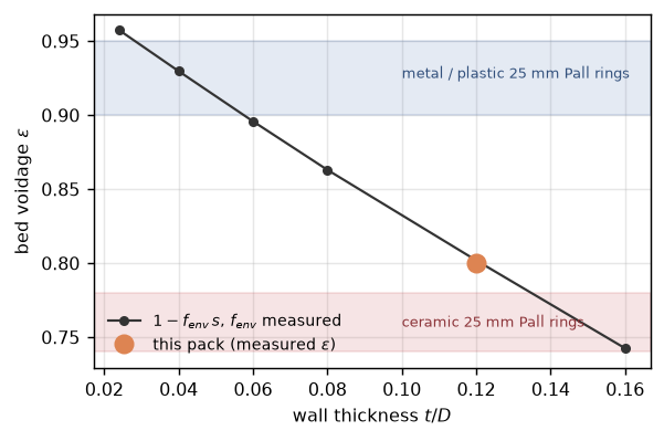
With one measured number — the envelope packing fraction of this pack — the same construction walks from our bed straight across the published range: 0.743 at \(t/D = 0.16\), squarely in the ceramic band, up to 0.957 at \(t/D = 0.024\) (a 0.6 mm sheet on a 25 mm ring), a little above the 0.90–0.95 quoted for metal rings. That last point overshooting is itself informative and not worth papering over: our bed is loose (\(\langle Z\rangle =\) 3.75, quasi-static), so \(f_{\text{env}}\) is on the low side, and a denser industrial pack would pull the whole curve down. The point stands regardless — the entire gap between \(\varepsilon =\) 0.800 and an industrial 0.94 is the wall, not the packing.
Step 7 — Freeze the pack
ni, nr, _, _ = b.encode()
np.savez_compressed(
"pall_ring_pack.npz",
positions=P.astype(np.float32), quaternions=Q.astype(np.float32),
box=np.array([L, L], np.float32), ring_volume=np.float32(sp.volume),
node_ints=np.asarray(ni, np.int32), node_reals=np.asarray(nr, np.float32),
home_root=np.int32(sp.home_root), bounding_radius=np.float32(sp.bounding_radius))
import os
print("pall_ring_pack.npz: %d rings, %.1f kB — the tree is stored too, so a consumer needs "
"nothing but this file." % (N, os.path.getsize("pall_ring_pack.npz") / 1024))
print("\ntotal page runtime %.0f s" % (time.time() - T_PAGE))
# Release the simulation's device allocations before the interpreter exits. Kokkos aborts if a
# View outlives Kokkos::finalize, and with a 1625-probe shell the contact buffers are large enough
# that the abort kills the Jupyter kernel mid-render rather than merely printing a backtrace.
import gc
del sim
gc.collect()pall_ring_pack.npz: 48 rings, 3.2 kB — the tree is stored too, so a consumer needs nothing but this file.
total page runtime 346 s3636Results
| claim | measured |
|---|---|
| certified tree: exterior probes violating Equation 1 | 0.00% (min slack +1.9e-12) |
| sign-exact tree, same solid: violations | 24.68% (worst ratio 0.7071) |
| ring solid volume / envelope cylinder | 0.3413 |
| surface area, specific surface | 6.561 \(D^2\), 8.35 \(/D\) |
| probe spacing (median) vs feature/3 | 0.0369 vs 0.0400 |
| bed voidage \(\varepsilon\) | 0.800 (0.0011 over three bulk windows) |
| envelope packing fraction \(f_{\text{env}}\) | 0.582 |
| mean coordination number | 3.75, 0 rattlers |
| ring-axis \(\lvert\cos\theta\rvert\) | 0.526 ± 0.042 (isotropic 0.500) |
| residual kinetic energy after the quench | 4.7e-04 of a one-diameter bed lift |
| max contact overlap | 0.027 = 23% of the wall; doubly-covered volume 0.0092% |
| \(\varepsilon\) predicted at \(t/D = 0.024\) / \(0.16\) | 0.957 / 0.743 vs published 0.90–0.95 / 0.74–0.78 |
The headline is the last row plus the second: the CSG ordering buys a certificate that a quarter of exterior queries would otherwise lose, and one measured envelope packing fraction carries the same construction across the published Pall-ring voidage range, from the ceramic band at \(t/D = 0.16\) to 0.957 at metal-sheet thickness — so the gap between this bed’s \(\varepsilon =\) 0.800 and an industrial 0.94 is geometric, not a packing failure.
Three caveats stated rather than buried. The bed is loose and quasi-static: mean coordination 3.75 sits at the isostatic ~4 rather than above it, so this is a marginally rigid bed rather than a jammed packing, and \(\varepsilon\) is correspondingly on the high side. The max contact overlap reaches 23% of the wall thickness — the price of a point-shell contact model on a thin, concave body — though the volume actually covered by two rings at once is only 0.0092% of the bed, so it does not move the porosity. And the bed does not come fully to rest: the quench leaves a residual jitter at 4.7e-04 of the bed’s gravitational scale, which is quasi-static, not static.
Adapt this yourself
- Change the packing element. Raschig ring: drop the windows and webs (
ring = tube). Berl saddle: intersect a torus with a half-space. Everything downstream — quadrature properties, principal frame, shell, contacts — follows with no other edit. - Keep the certificate. Whenever you subtract, put the certified leaf on the left. Check it the way Step 2 does; an uncertified instance is never pruned, so it costs a full evaluation on every query.
- Change the wall thickness and re-run the pour, rather than the sweep: Equation 2 assumes \(f_{\text{env}}\) is thickness-independent, which is a hypothesis this page does not test.
- Push flow through it. The frozen
.npzcarries the tree, so the pack can be handed topeclet.flowas scene instances for a pressure-drop calculation.
Reproduce this
# from PyPI (needs a peclet newer than the current release — see the note at the top)
pip install peclet scikit-image
quarto render examples/pall-ring-packing/index.qmd --execute
# from a local suite build
PECLET_LOCAL_BUILD=/path/to/suite/dem/build_l4_omp:/path/to/suite/core/python/build_geom \
OMP_NUM_THREADS=8 OMP_PROC_BIND=false \
quarto render examples/pall-ring-packing/index.qmd --executeReferences
Billet, Reinhard, and Michael Schultes. 1999. “Prediction of Mass Transfer Columns with Dumped and Arranged Packings: Updated Summary of the Calculation Method of Billet and Schultes.” Chemical Engineering Research and Design 77 (6): 498–504. https://doi.org/10.1205/026387699526520.
Stichlmair, J., J. L. Bravo, and J. R. Fair. 1989. “General Model for Prediction of Pressure Drop and Capacity of Countercurrent Gas/Liquid Packed Columns.” Gas Separation & Purification 3 (1): 19–28. https://doi.org/10.1016/0950-4214(89)80016-7.