# Makes this notebook run out-of-the-box on Colab/Binder. A real user just needs the
# published package; this installs it on first run. Authors can instead point at a
# local source build of the suite with the PECLET_LOCAL_BUILD env var.
import importlib.util, os, subprocess, sys
_local = os.environ.get("PECLET_LOCAL_BUILD")
if _local:
    sys.path.insert(0, _local)                                  # local source build
elif importlib.util.find_spec("peclet") is None:
subprocess.run([sys.executable, "-m", "pip", "install", "-q", "peclet", "mpmath"], check=True)Capillary oscillations: a wave and a drop against exact viscous theory
Surface tension as a restoring force, measured two ways — and what changes when the reference is the exact viscous normal mode instead of the inviscid textbook formula.
flow
vof
two-phase
surface-tension
verification
 Five runs of one to three thousand steps each — minutes on a GPU build, slow but possible on a Colab CPU runtime.
What you’ll learn
The parasitic-currents page showed that peclet’s surface-tension force is statically exact. This page asks the harder question: does it produce the right dynamics — the right frequency and the right damping when the interface is released and allowed to ring?
Two classical normal modes answer it, and they answer it differently:
- A standing capillary wave matches the exact viscous two-fluid dispersion relation to better than 0.6 % in frequency at 32 and 64 cells per wavelength. Compared against the inviscid formula the same runs read \(-2\ldots-4\,\%\) — so the “deviation” an earlier campaign recorded was the reference, not the solver. The damping likewise: the two-fluid rate is the \(O(\sqrt{\nu})\) interfacial boundary-layer rate, several times larger than the free-surface \(2\nu k^2\) that gets quoted for it (1.7–3.9× over the three rungs here).
- A mode-2 droplet does not close the same way. Against Lamb it is 5–6 % low; the exact viscous shift explains about 2 % of that at \(\mu=0.0025\) and 5 % at \(\mu=0.02\) — and the simulation captures only part of even that, because its interfacial boundary layer is a fraction of a cell wide. What survives is an inviscid deficit of about 4 % that does not shrink with resolution and that the campaign has not attributed. We state it as an open measured deviation and list what it is not.
Along the way: how to measure \(\omega\) and \(\gamma\) from a short, noisy, damped series without lying to yourself — a two-extremum ratio is an upper bound, a damped-sinusoid least-squares fit is a measurement.
The conclusion to carry away: picking the right reference is half of a verification. One of these two benchmarks passes cleanly once you do; the other still doesn’t, and that is worth publishing too.
The problem: two normal modes of surface tension
Both cases are the same physics — an interface displaced from its minimum-area shape, released from rest, ringing under surface tension against the inertia of the fluid on both sides, and losing amplitude to viscosity. Both are linear normal modes \(\propto e^{st}\), with \(s = -\gamma + i\omega\). Both are run with matched fluids (equal density \(\rho\), equal kinematic viscosity \(\nu\)) so the only contrast in the problem is the surface tension itself — which makes the exact references clean and removes density-ratio conditioning from the pressure solve.
A. The planar standing wave
A flat interface at mid-height carries a small cosine perturbation of wavenumber \(k = 2\pi/\lambda\). The inviscid dispersion relation for two semi-infinite fluids of equal density (Lamb 1932, art. 267) is
\[ \omega_0^2 = \frac{\sigma k^3}{\rho_1+\rho_2} = \frac{\sigma k^3}{2\rho} , \tag{1}\]
and with walls a distance \(H\) above and below the interface the added-mass factor \(\tanh(kH)\) multiplies it (\(0.4\,\%\) at \(kH=\pi\), which is this page’s geometry). The damping rate usually quoted alongside it, \(\gamma = 2\nu k^2\), is the rate for a free surface — a liquid with a vacuum above. It is the wrong rate here.
For two viscous fluids the mode is not a lightly damped version of Equation 1 at all; the vorticity generated at the interface diffuses into a boundary layer of thickness \(\sqrt{\nu/\omega_0}\) and the correct normal-mode condition (Prosperetti 1981) is transcendental:
\[ s^2 + \omega_0^2\!\left(1 - \frac{k}{\sqrt{k^2 + s/\nu}}\right) = 0 , \qquad \operatorname{Re}\sqrt{\cdot} > 0 . \tag{2}\]
Where it comes from. With equal fluids the vertical velocity amplitude is even about the interface, \(\hat w(z) = A e^{-k|z|} + B e^{-m|z|}\) with \(m^2 = k^2 + s/\nu\). Continuity of \(\hat w\), \(\hat w'\) and \(\hat w''\) across the interface fixes \(B/A\), and the normal-stress jump — which is where surface tension enters — reads \(\mu[\hat w'''] = -\sigma k^4 \hat w(0)/s\). Eliminating \(A\) and \(B\) gives Equation 2. Expanding to first order in \(\varepsilon = k\sqrt{\nu/\omega_0}\),
\[ s = i\omega_0 - (1+i)\,\frac{\omega_0\varepsilon}{2\sqrt 2} \quad\Longrightarrow\quad \frac{\Delta\omega}{\omega_0} = -\frac{\gamma}{\omega_0} = -\frac{k}{2\sqrt2}\sqrt{\frac{\nu}{\omega_0}} . \tag{3}\]
Two things fall out of that one line. The frequency deficit is \(O(\sqrt\nu)\), not \(O(\nu)\) — an order of magnitude bigger than the weak-damping estimate \((\gamma/\omega)^2/2\) that a free-surface intuition suggests. And the damping equals that deficit, so any code whose frequency sits a few percent below Equation 1 should check Equation 2 before blaming its discretization.
B. The mode-2 drop
A sphere of radius \(R\) is deformed into a prolate spheroid at constant volume and released. Lamb’s inviscid frequency (Lamb 1932, art. 275) for mode \(n\) is
\[ \omega_0^2 = \frac{n(n-1)(n+1)(n+2)\,\sigma}{R^3\big[(n+1)\rho_{\text{in}} + n\rho_{\text{out}}\big]} \;\xrightarrow[\ \rho_{\text{in}}=\rho_{\text{out}}=\rho\ ]{n=2}\; \frac{24\,\sigma}{5\rho R^3} . \tag{4}\]
The viscous version is Miller & Scriven’s (Miller and Scriven 1968) unsteady-Stokes normal mode. Inside and outside, the velocity splits into a potential part (\(r^n\) inside, \(r^{-(n+1)}\) outside) and a poloidal vortical part (\(j_n(qr)\) inside, \(h_n^{(1)}(qr)\) outside, with \(q^2 = -s/\nu\) and \(\operatorname{Im} q > 0\) so the outer solution decays). Matching at \(r=R\) the radial velocity, the tangential velocity, the shear stress \(\tau_{r\theta}\), and the normal-stress jump \(\sigma(n-1)(n+2)\eta/R^2\) with \(s\eta = u_r\), gives a \(4\times4\) determinant whose root near \(i\omega_0\) is the mode. To first order in \(\sqrt{\nu/(\omega_0 R^2)}\) the \(n=2\) shift is
\[ \frac{\Delta\omega}{\omega_0} = -0.885\,\sqrt{\frac{\nu}{\omega_0 R^2}} , \tag{5}\]
again \(O(\sqrt\nu)\) and again equal in magnitude to the damping at leading order.
import math
import numpy as np
import matplotlib.pyplot as plt
from scipy.optimize import fsolve, least_squares
from peclet import flow

plt.rcParams.update({"figure.dpi": 130, "font.size": 10, "axes.grid": True,
                     "grid.alpha": 0.3, "axes.axisbelow": True,
                     "figure.facecolor": "white", "savefig.bbox": "tight"})
BLUE, RED, GREY, GREEN, ORANGE = "#1f77b4", "#d62728", "0.80", "#2ca02c", "#ff7f0e"
The exact references, in twenty lines each
These are the yardsticks, and they are short enough to read. The wave root is a two-dimensional Newton solve on Equation 2; the drop root is the \(4\times4\) determinant of the previous section, evaluated in mpmath because the spherical Hankel functions of a complex argument underflow badly in double precision (hence the column scaling by \(j_n(qR)\) and \(h_n(qR)\), which does not move the root).
def wave_mode(k, nu, sigma=1.0, rho=1.0, H=None):
    """Complex growth rate s of the two-fluid capillary wave: eq-wave-exact.

    Re s < 0 is the decay rate, Im s the angular frequency. H = wall half-distance."""
    w0sq = sigma * k ** 3 / (2 * rho)
    if H is not None:
        w0sq *= math.tanh(k * H)                 # finite depth: added mass of the walls
    w0 = math.sqrt(w0sq)

    def f(v):
        s = complex(v[0], v[1])
        m = np.sqrt(k * k + s / nu)
        if m.real < 0:
            m = -m                               # the branch that decays away from z = 0
        r = s * s + w0sq * (1.0 - k / m)
        return [r.real, r.imag]

    eps = k * math.sqrt(nu / w0)                 # eq-wave-first as the initial guess
    v = fsolve(f, [-w0 * eps / (2 * math.sqrt(2)),
                   w0 * (1 - eps / (2 * math.sqrt(2)))], xtol=1e-12)
    return complex(v[0], v[1]), w0


def drop_mode(n, R, nu, sigma=1.0, rho=1.0, dps=50):
    """Complex growth rate s of mode n of a drop in an IDENTICAL fluid (Miller & Scriven).

    Returns (s, omega_0) with omega_0 Lamb's inviscid frequency, eq-lamb."""
    import mpmath as mp
    mp.mp.dps = dps
    mu = rho * nu

    def jn(z):                                    # spherical Bessel / Hankel of order n
        return mp.sqrt(mp.pi / (2 * z)) * mp.besselj(n + mp.mpf(1) / 2, z)

    def hn(z):
        return mp.sqrt(mp.pi / (2 * z)) * mp.hankel1(n + mp.mpf(1) / 2, z)

    def det(s):
        q = mp.sqrt(-s / nu)
        if mp.im(q) < 0:
            q = -q                                # the outer vortical solution must decay
        Rm = mp.mpf(R)
        jR, hR = jn(q * Rm), hn(q * Rm)           # root-neutral column scaling
        basis = [(lambda r: (r / Rm) ** n, lambda r: mp.mpf(0), 1),        # potential, in
                 (lambda r: mp.mpf(0), lambda r: jn(q * r) / jR, 1),       # vortical, in
                 (lambda r: (Rm / r) ** (n + 1), lambda r: mp.mpf(0), -1), # potential, out
                 (lambda r: mp.mpf(0), lambda r: hn(q * r) / hR, -1)]      # vortical, out
        M = mp.matrix(4, 4)
        for j, (phi, f, sg) in enumerate(basis):
            U = lambda x, phi=phi, f=f: mp.diff(phi, x) + n * (n + 1) * f(x) / x   # u_r
            V = lambda x, phi=phi, f=f: (phi(x) + mp.diff(lambda y: y * f(y), x)) / x
            T = mu * (Rm * mp.diff(lambda y: V(y) / y, Rm) + U(Rm) / Rm)          # tau_rt
            N = rho * s * phi(Rm) + 2 * mu * mp.diff(U, Rm)                       # normal
            M[0, j], M[1, j], M[2, j] = sg * U(Rm), sg * V(Rm), sg * T
            M[3, j] = (-sg * N - (sigma * (n - 1) * (n + 2) / (s * Rm ** 2))
                       * U(Rm) * (1 if sg == 1 else 0))
        return mp.det(M)

    w0 = mp.sqrt(n * (n - 1) * (n + 1) * (n + 2) * sigma / (R ** 3 * (2 * n + 1) * rho))
    eps = mp.sqrt(nu / (w0 * R * R))
    s0 = w0 * mp.mpc(-0.885 * eps, 1 - 0.885 * eps)          # eq-drop-first as the guess
    d0 = det(s0)
    s = mp.findroot(lambda s: det(s) / d0, s0, tol=1e-24, maxsteps=200)
    return complex(s), float(w0)
Measuring \(\omega\) and \(\gamma\) from a short damped series
Reading a frequency off the zero crossings is safe: it is a set of independent half-period measurements and averaging them is unbiased. Reading a decay rate off the ratio of two successive extrema is not — an initial-value problem released from rest is not a pure exponential from step one (the boundary layer has to establish itself; that is exactly why Prosperetti’s Laplace-transform solution exists), so the first extremum is too high and the two-extremum estimate is an upper bound rather than a measurement.
The honest estimator uses the whole record. We fit
\[ a(t) \approx A\,e^{-\gamma t}\cos(\omega t + \varphi) + B \tag{6}\]
by nonlinear least squares, skipping the first quarter period so the start-up transient does not set the parameters. Both estimators are reported below so you can see the difference for yourself.
def zero_crossings(t, y):
    """Times of the sign changes of y (linear interpolation)."""
    out = []
    for i in range(len(y) - 1):
        if y[i] == 0.0:
            out.append(t[i])
        elif y[i] * y[i + 1] < 0.0:
            out.append(t[i] + (t[i + 1] - t[i]) * y[i] / (y[i] - y[i + 1]))
    return np.array(out)


def damped_fit(t, y, w_guess, skip_periods=0.25):
    """Least-squares fit of eq-fit. Returns omega, gamma, the baseline B and the fitted curve."""
    m = t >= t[0] + skip_periods * (2 * math.pi / w_guess)   # skip the start-up transient
    tt, yy = t[m], y[m]

    def model(p, x):
        A, g, w, ph, B = p
        return A * np.exp(-g * (x - tt[0])) * np.cos(w * (x - tt[0]) + ph) + B

    a0 = float(np.max(np.abs(yy - np.mean(yy)))) or 1.0
    p0 = [a0, 1e-3, w_guess, 0.0, float(np.mean(yy))]
    r = least_squares(lambda p: model(p, tt) - yy, p0,
                      x_scale=[a0, 1e-3, w_guess, 1.0, a0])
    A, g, w, ph, B = r.x
    return dict(omega=abs(w), gamma=g, offset=B, amp=abs(A), curve=(tt, model(r.x, tt)))


def omega_from_crossings(t, y, baseline):
    """Independent frequency estimate: pi over the mean half-period between sign changes."""
    zc = zero_crossings(t, y - baseline)
    return math.pi / np.mean(np.diff(zc)) if len(zc) >= 3 else float("nan")


def gamma_two_extrema(t, y, baseline):
    """The first/last-extremum ratio: an UPPER bound on the decay rate, not a measurement."""
    y = y - baseline
    pk = [i for i in range(1, len(y) - 1)
          if abs(y[i]) > abs(y[i - 1]) and abs(y[i]) > abs(y[i + 1])]
    if len(pk) < 2:
        return float("nan")
    return -math.log(abs(y[pk[-1]]) / abs(y[pk[0]])) / (t[pk[-1]] - t[pk[0]])


class Solve:
    """A run's solver health: pressure iterations against the cap, and flux divergence."""

    def __init__(self, cap):
        self.cap, self.iters, self.div = cap, 0, 0.0

    def sample(self, s):
        self.iters = max(self.iters, s.last_pressure_iterations())
        self.div = max(self.div, s.max_open_divergence())

    @property
    def valid(self):
        return self.iters < self.cap

    def __str__(self):
        return (f"pressure {self.iters}/{self.cap}"
                f"{'' if self.valid else '  *** CAPPED -> RUN INVALID ***'}, "
                f"max|div| {self.div:.1e}")
ImportantA run whose pressure solve hit its iteration cap is not a result
Every run on this page records last_pressure_iterations() against its cap and max_open_divergence(), and prints both. A capped solve means the projection did not converge, the velocity field is not discretely divergence-free, and a frequency measured on it is an artefact of the linear solver. None of the runs below capped.
Part A — the standing capillary wave
The setup is quasi-2D: \(n_x \times 4 \times n_x\) cells, periodic in \(x\) and \(y\), walls at \(\pm z\), a flat interface at mid-height carrying one full wavelength \(\lambda = L_x\) of cosine perturbation with amplitude \(a_0 = \lambda/100\). Solver units throughout: the cell is 1, \(\sigma = \rho = 1\).
The initial condition is the one thing worth being careful about. VoF wants the exact volume fraction of liquid in each cell, and for a single-valued interface \(z = z_i(x)\) that is available in closed form: integrate the interface height across the cell’s \(x\)-extent analytically, \(\bar z_i = \tfrac{1}{h}\!\int \! z_i\,dx\), and clip \(\bar z_i - k\) into \([0,1]\) for cell row \(k\). Sampling a level set at cell centres instead would put an \(O(h)\) error into the very shape whose curvature drives the mode.
def capillary_wave(nx, nu, periods=2.5, rho=1.0, sigma=1.0, cls=flow.Solver):
    """Standing capillary wave of wavelength lambda = nx cells; returns amplitude(t).

    `cls` is the solver class -- the collocated cross-check at the end passes
    flow.SolverColocated; everything else is identical."""
    nz, ny = nx, 4
    lam = float(nx)
    k = 2 * math.pi / lam
    a0 = lam / 100.0

    s = cls(nx, ny, nz)
    s.set_rho(rho)
    s.set_mu(nu * rho)
    s.set_domain_bc(4, 1, 0, 0, 0)                     # -z wall
    s.set_domain_bc(5, 1, 0, 0, 0)                     # +z wall
    s.set_pressure_geometry(np.full((nx, ny, nz), 10.0, order="F"))
    s.set_pressure_chebyshev(True, 500, 1e-11)
    s.enable_vof()

    xe = np.arange(nx + 1)                             # exact fractions of z = nz/2 + a0 cos kx
    zi = nz / 2.0 + a0 * (np.sin(k * xe[1:]) - np.sin(k * xe[:-1])) / k
    C = np.zeros((nx, ny, nz))
    for kk in range(nz):
        C[:, :, kk] = np.clip(zi - kk, 0.0, 1.0)[:, None]
    s.set_vof(np.asfortranarray(C))
    s.set_property_model("rho", "linear", "C", [rho, 0.0])   # matched fluids
    s.set_surface_tension(sigma)
    dt = 0.5 * s.capillary_dt()
    s.set_dt(dt)

    w_inv = math.sqrt(sigma * k ** 3 / (2 * rho))
    nsteps = int(periods * 2 * math.pi / w_inv / dt)
    h, t, amp = Solve(500), [], []
    cosx = np.cos(k * (np.arange(nx) + 0.5))
    for i in range(nsteps):
        s.step()
        h.sample(s)
        col = s.get_vof().sum(axis=2)[:, 0]            # column sum = interface height, exactly
        t.append((i + 1) * dt)
        amp.append(float(np.dot(col - nz / 2.0, cosx) * 2.0 / nx))
    return dict(nx=nx, nu=nu, k=k, a0=a0, dt=dt, nsteps=nsteps, health=h,
                t=np.array(t), amp=np.array(amp))
The amplitude is the projection of the interface height onto the mode, \(a(t) = \frac{2}{n_x}\sum_i (\textstyle\sum_k C_{ik} - n_z/2)\cos k x_i\) — not a peak height. For a single-valued interface the column sum of \(C\) is the height, exactly, so this costs nothing and rejects every other Fourier component.
WAVE = [(32, 0.005), (64, 0.005), (32, 0.02)]
waves = [capillary_wave(nx, nu) for nx, nu in WAVE]
for r in waves:
    s_ex, w0_H = wave_mode(r["k"], r["nu"], H=r["nx"] / 2.0)
    r["s_exact"], r["w0_H"] = s_ex, w0_H
    r["w_inviscid"] = math.sqrt(r["k"] ** 3 / 2.0)
    f = damped_fit(r["t"], r["amp"], r["w_inviscid"])
    r["w_fit"], r["g_fit"], r["curve"] = f["omega"], f["gamma"], f["curve"]
    r["base"] = f["offset"]                                # the fit's own baseline...
    r["w_zc"] = omega_from_crossings(r["t"], r["amp"], r["base"])       # ...used by the
    r["g_2e"] = gamma_two_extrema(r["t"], r["amp"], r["base"])          # other two estimators
    print(f"{r['nx']:>3} cells/lambda, nu = {r['nu']:<6g} {r['nsteps']:>5} steps, "
          f"dt = {r['dt']:.3f}; {r['health']}")
32 cells/lambda, nu = 0.005 1280 steps, dt = 0.199; pressure 12/500, max|div| 2.0e-15
64 cells/lambda, nu = 0.005 3620 steps, dt = 0.199; pressure 11/500, max|div| 1.7e-15
32 cells/lambda, nu = 0.02 1280 steps, dt = 0.199; pressure 12/500, max|div| 2.0e-15Frequency: against the inviscid formula, and against the exact root
print(f"{'cells/l':>8} {'nu':>7} | {'omega fit':>10} {'omega zc':>9} | "
      f"{'inviscid':>9} {'err':>8} | {'exact':>9} {'err (fit)':>10} {'err (zc)':>9}")
for r in waves:
    print(f"{r['nx']:>8} {r['nu']:>7g} | {r['w_fit']:>10.5f} {r['w_zc']:>9.5f} | "
          f"{r['w_inviscid']:>9.5f} {100*(r['w_fit']/r['w_inviscid']-1):>7.2f}% | "
          f"{r['s_exact'].imag:>9.5f} {100*(r['w_fit']/r['s_exact'].imag-1):>9.2f}% "
          f"{100*(r['w_zc']/r['s_exact'].imag-1):>8.2f}%")
cells/l nu | omega fit omega zc | inviscid err | exact err (fit) err (zc)
32 0.005 | 0.06018 0.06016 | 0.06152 -2.19% | 0.06019 -0.02% -0.04%
64 0.005 | 0.02131 0.02130 | 0.02175 -2.04% | 0.02135 -0.19% -0.22%
32 0.02 | 0.05929 0.05927 | 0.06152 -3.63% | 0.05897 0.54% 0.50%Damping: the free-surface rate is not this problem’s rate
print(f"{'cells/l':>8} {'nu':>7} | {'gamma fit':>10} {'2 extrema':>10} | "
      f"{'2 nu k^2':>10} {'x':>6} | {'exact':>10} {'err (fit)':>10}")
for r in waves:
    g_fs = 2 * r["nu"] * r["k"] ** 2
    g_ex = -r["s_exact"].real
    print(f"{r['nx']:>8} {r['nu']:>7g} | {r['g_fit']:>10.3e} {r['g_2e']:>10.3e} | "
          f"{g_fs:>10.3e} {g_ex/g_fs:>5.1f}x | {g_ex:>10.3e} "
          f"{100*(r['g_fit']/g_ex-1):>9.1f}%")
cells/l nu | gamma fit 2 extrema | 2 nu k^2 x | exact err (fit)
32 0.005 | 1.083e-03 1.075e-03 | 3.855e-04 3.3x | 1.264e-03 -14.3%
64 0.005 | 4.633e-04 4.606e-04 | 9.638e-05 3.9x | 3.737e-04 24.0%
32 0.02 | 2.730e-03 2.711e-03 | 1.542e-03 1.7x | 2.625e-03 4.0%from matplotlib.lines import Line2D
fig, (ax, axb) = plt.subplots(1, 2, figsize=(8.4, 3.3),
gridspec_kw=dict(width_ratios=[1.55, 1.0], wspace=0.32))
for r, c in zip(waves, (BLUE, GREEN, RED)):
T = 2 * math.pi / r["s_exact"].imag
ax.plot(r["t"] / T, r["amp"] / r["a0"], color=c, lw=1.4,
label=rf"{r['nx']} cells/$\lambda$, $\nu$ = {r['nu']:g}")
tt, yy = r["curve"]
ax.plot(tt / T, yy / r["a0"], color="0.2", lw=1.0, ls=(0, (4, 3)), zorder=4)
ax.axhline(0, color="0.5", lw=0.8)
ax.set(xlabel=r"$t\,/\,T_{\rm exact}$", ylabel=r"mode amplitude $a(t)/a_0$",
title="Standing capillary wave", ylim=(-1.62, 1.28))
handles = ax.get_legend_handles_labels()[0]
handles.append(Line2D([], [], color="0.2", lw=1.0, ls=(0, (4, 3))))
ax.legend(handles, [rf"{r['nx']} cells/$\lambda$, $\nu$ = {r['nu']:g}" for r in waves]
+ [r"fitted $Ae^{-\gamma t}\cos(\omega t+\varphi)+B$"],
fontsize=7.5, loc="lower center", ncol=2, frameon=False)
x = np.arange(len(waves))
e_inv = np.array([100 * (r["w_fit"] / r["w_inviscid"] - 1) for r in waves])
e_ex = np.array([100 * (r["w_fit"] / r["s_exact"].imag - 1) for r in waves])
axb.bar(x - 0.19, e_inv, 0.36, color="0.65", label="vs the inviscid formula")
axb.bar(x + 0.19, e_ex, 0.36, color=BLUE, label="vs the exact viscous root")
for xi, v, col in ([(xi, v, "0.35") for xi, v in zip(x - 0.19, e_inv)]
+ [(xi, v, BLUE) for xi, v in zip(x + 0.19, e_ex)]):
axb.text(xi, v - 0.10 if v < 0 else v + 0.10, f"{v:+.2f}", ha="center",
va="top" if v < 0 else "bottom", fontsize=8, color=col)
axb.axhline(0, color="0.3", lw=0.9)
axb.set_xticks(x)
axb.set_xticklabels([f"{r['nx']}\n$\\nu$={r['nu']:g}" for r in waves], fontsize=8)
axb.set(ylabel="frequency error [%]", title="Which reference you use",
ylim=(1.55 * e_inv.min(), max(1.0, 2.2 * e_ex.max())))
axb.legend(fontsize=7.5, loc="lower left", frameon=False)
axb.grid(axis="x", visible=False)
plt.show()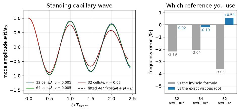
The headline. Against the exact viscous root the measured frequencies are within 0.54 % — the individual rungs read -0.02 %, -0.19 %, +0.54 % at 32/64/32 cells per wavelength. Against Equation 1 the same three runs read -2.19 %, -2.04 %, -3.63 %, which is the “\(-2\ldots-4\,\%\) deviation” an earlier pass of this benchmark recorded and could not explain. It was the reference. Note the diagnostic that gives it away and costs nothing: the deficit grows with \(\nu\) (the \(\nu = 0.02\) rung is worst), which no consistent spatial discretization error does, and which Equation 3 predicts exactly.
The damping is the other half of the same statement. The exact rate is 1.7–3.9 times the free-surface \(2\nu k^2\) at these parameters, because the two-fluid mode dissipates in an interfacial boundary layer of thickness \(\sqrt{\nu/\omega_0}\) rather than in the bulk: an \(O(\sqrt\nu)\) rate against an \(O(\nu)\) one. Measured against that rate, the fitted decay lands within 24 % — the accuracy a two-and-a-half-period envelope supports, and a far weaker statement than the frequency’s. The two-extremum ratio is printed beside it: over this short a record the two estimators land close together, which says the envelope is nearly exponential after the transient, not that either is accurate.
NoteWhy the damping is harder to measure than the frequency
The frequency comes from many independent half-periods; the decay comes from an amplitude envelope observed over only 2.5 periods, on a signal that is not a pure exponential at the start. A few percent of the initial amplitude going into the boundary-layer transient moves \(\gamma\) by tens of percent while moving \(\omega\) by nothing. That is why this page quotes both estimators, and why the frequency — not the decay — is the sharp test.
Part B — the mode-2 droplet
Now the curved interface. A sphere of radius \(R = 8\) cells is initialised as a prolate spheroid at constant volume, \(a = R(1+\varepsilon)\), \(b = c = R/\sqrt{1+\varepsilon}\) with \(\varepsilon = 0.05\), in a \(48^3\) periodic box — a drop-to-box volume ratio of \(\varphi \approx 1.9\,\%\), eight times smaller than the earlier campaign’s \(32^3\) setup, which is how confinement was ruled out. Released from rest, it rings in mode 2.
The observable is the \(P_2\) shape moment of the colour field,
\[ m_2(t) = \big\langle\, 2z^2 - x^2 - y^2 \,\big\rangle_C = \frac{\sum_{ijk} C_{ijk}\,\big(2z_k^2-x_i^2-y_j^2\big)}{\sum_{ijk} C_{ijk}} , \tag{7}\]
which is exactly the mode’s own projection: it is blind to translation of the drop, to volume drift, and to every shape harmonic except \(n=2\). (The campaign checked it against two independent shape measures — the polar half-height and the equatorial half-width — which give the same frequency to within 0.6 %.)
def oscillating_drop(n, R, mu, eps=0.05, periods=2.5, rho=1.0, sigma=1.0, cls=flow.Solver):
    """Mode-2 oscillation of a drop of radius R cells in an n^3 periodic box of the SAME fluid.

    `cls` is the solver class (see the collocated cross-check at the end)."""
    a, b = R * (1 + eps), R / math.sqrt(1 + eps)         # prolate, volume-preserving
    cx = cy = cz = n / 2 + 0.137                         # off-symmetry placement
    sub = 16
    ax = (np.arange(n)[:, None] + (np.arange(sub)[None, :] + 0.5) / sub).ravel()
    X, Y = ax[:, None], ax[None, :]
    half = a * np.sqrt(np.maximum(1.0 - ((X - cx) ** 2 + (Y - cy) ** 2) / b ** 2, 0.0))
    C = np.zeros((n, n, n))                              # exact in z, subsampled in (x, y)
    for kk in range(n):
        seg = np.maximum(np.minimum(cz + half, kk + 1) - np.maximum(cz - half, kk), 0.0)
        C[:, :, kk] = seg.reshape(n, sub, n, sub).mean(axis=(1, 3))

    s = cls(n, n, n)
    s.set_rho(rho)
    s.set_mu(mu)
    s.set_pressure_geometry(np.full((n, n, n), 10.0, order="F"))
    s.set_pressure_chebyshev(True, 500, 1e-11)
    s.enable_vof()
    s.set_vof(np.asfortranarray(C))
    s.set_property_model("rho", "linear", "C", [rho, 0.0])    # matched fluids
    s.set_surface_tension(sigma)
    dt = 0.5 * s.capillary_dt()
    s.set_dt(dt)

    w0 = math.sqrt(24 * sigma / (5 * rho * R ** 3))           # eq-lamb, n = 2, equal densities
    nsteps = int(periods * 2 * math.pi / w0 / dt)
    xs, ys, zs = ((np.arange(n) + 0.5) - c for c in (cx, cy, cz))
    P2 = 2 * zs[None, None, :] ** 2 - xs[:, None, None] ** 2 - ys[None, :, None] ** 2
    h, t, m2, vol = Solve(500), [], [], []
    for i in range(nsteps):
        s.step()
        h.sample(s)
        Cf = s.get_vof()
        v = Cf.sum()
        t.append((i + 1) * dt)
        m2.append(float((Cf * P2).sum() / v))
        vol.append(float(v))
    return dict(n=n, R=R, mu=mu, dt=dt, nsteps=nsteps, health=h, w0=w0,
                t=np.array(t), m2=np.array(m2), vol=np.array(vol),
                branch=s.vof_curvature_branch(), kappa=s.vof_curvature())
DROPS = [0.0025, 0.02]
drops = [oscillating_drop(48, 8.0, mu) for mu in DROPS]
for r in drops:
s_ex, w0 = drop_mode(2, r["R"], r["mu"]) # nu = mu, since rho = 1
r["s_exact"] = s_ex
f = damped_fit(r["t"], r["m2"], r["w0"])
r["w_fit"], r["g_fit"], r["curve"] = f["omega"], f["gamma"], f["curve"]
r["base"] = f["offset"]
r["w_zc"] = omega_from_crossings(r["t"], r["m2"], r["base"])
print(f"mu = {r['mu']:<7g} {r['nsteps']:>5} steps, dt = {r['dt']:.3f}; {r['health']}; "
f"volume drift {r['vol'][-1]/r['vol'][0]-1:+.1e}")mu = 0.0025 813 steps, dt = 0.199; pressure 10/500, max|div| 7.1e-13; volume drift -1.4e-14
mu = 0.02 813 steps, dt = 0.199; pressure 10/500, max|div| 7.1e-13; volume drift -1.4e-14print(f"{'mu':>7} {'delta/h':>8} | {'omega fit':>10} {'omega zc':>9} | "
f"{'Lamb':>9} {'err':>8} | {'exact visc':>11} {'shift':>7} {'err':>8}")
for r in drops:
ex = r["s_exact"]
delta = math.sqrt(r["mu"] / r["w0"]) # interfacial boundary layer, cells
print(f"{r['mu']:>7g} {delta:>8.2f} | {r['w_fit']:>10.5f} {r['w_zc']:>9.5f} | "
f"{r['w0']:>9.5f} {100*(r['w_fit']/r['w0']-1):>7.2f}% | "
f"{ex.imag:>11.5f} {100*(ex.imag/r['w0']-1):>6.2f}% "
f"{100*(r['w_fit']/ex.imag-1):>7.2f}%")
print()
print(f"{'mu':>7} | {'gamma fit':>10} | {'exact visc':>11} {'err':>8} "
f"(the mode's own damping)")
for r in drops:
g_ex = -r["s_exact"].real
print(f"{r['mu']:>7g} | {r['g_fit']:>10.3e} | {g_ex:>11.3e} "
f"{100*(r['g_fit']/g_ex-1):>7.1f}%") mu delta/h | omega fit omega zc | Lamb err | exact visc shift err
0.0025 0.16 | 0.09142 0.09142 | 0.09682 -5.58% | 0.09511 -1.78% -3.87%
0.02 0.45 | 0.09072 0.09079 | 0.09682 -6.30% | 0.09196 -5.03% -1.34%
mu | gamma fit | exact visc err (the mode's own damping)
0.0025 | 1.472e-03 | 1.780e-03 -17.3%
0.02 | 4.463e-03 | 5.350e-03 -16.6%fig, (ax, axb) = plt.subplots(1, 2, figsize=(8.4, 3.3),
gridspec_kw=dict(width_ratios=[1.55, 1.0], wspace=0.32))
for r, c in zip(drops, (BLUE, RED)):
T = 2 * math.pi / r["w0"]
base = r["base"]
ax.plot(r["t"] / T, (r["m2"] - base) / abs(r["m2"][0] - base), color=c, lw=1.4,
label=rf"$\mu$ = {r['mu']:g}, $\sqrt{{\nu/\omega_0}}$ = "
rf"{math.sqrt(r['mu']/r['w0']):.2f} cells")
tt, yy = r["curve"]
ax.plot(tt / T, (yy - base) / abs(r["m2"][0] - base), color="0.25", lw=1.0, ls="--",
zorder=4)
ax.axhline(0, color="0.5", lw=0.8)
ax.set(xlabel=r"$t\,/\,T_{\rm Lamb}$", ylabel=r"$P_2$ moment (normalised)",
title=r"Mode-2 drop, $48^3$, $R = 8$", ylim=(-1.55, 1.25))
ax.legend(fontsize=8, loc="lower center", frameon=False)
x = np.arange(len(drops))
tot = np.array([100 * (r["w_fit"] / r["w0"] - 1) for r in drops])
visc = np.array([100 * (r["s_exact"].imag / r["w0"] - 1) for r in drops])
res = tot - visc
axb.bar(x, visc, 0.45, color=BLUE, label="exact viscous shift")
axb.bar(x, res, 0.45, bottom=visc, color="white", edgecolor=RED, hatch="///",
label="left over after subtracting it")
for xi, t_, v, rr in zip(x, tot, visc, res):
axb.text(xi, v / 2, f"{v:.1f}", ha="center", va="center", fontsize=8, color="white")
axb.text(xi, v + rr / 2, f"{rr:.1f}", ha="center", va="center", fontsize=8, color=RED)
axb.text(xi, t_ - 0.16, f"total {t_:.1f} %", ha="center", va="top", fontsize=8.5)
axb.axhline(0, color="0.3", lw=0.9)
axb.set_xticks(x)
axb.set_xticklabels([rf"$\mu$ = {r['mu']:g}" for r in drops])
axb.set(ylabel="frequency deficit vs Lamb [%]", title="What the deficit is made of",
ylim=(1.42 * tot.min(), 0.45))
axb.legend(fontsize=7.5, loc="lower center", frameon=False)
axb.grid(axis="x", visible=False)
plt.show()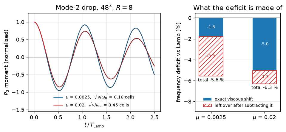
The numbers, stated plainly. At \(48^3\) with \(R = 8\) the measured mode-2 frequency is -5.6 %, -6.3 % below Lamb at \(\mu =\) 0.0025, 0.02. The exact viscous mode accounts for -1.8 %, -5.0 % of it. Subtracting the one from the other leaves -3.8 %, -1.3 %.
Those two residuals are not directly comparable, and the reason is worth following, because it is the difference between a number and a claim. The simulation does not capture the whole viscous shift it is being credited with: its fitted damping is -17 %, -17 % relative to the exact rate, because the interfacial boundary layer \(\sqrt{\nu/\omega_0}\) is only 0.16, 0.45 cells thick here. A sub-cell boundary layer is not resolved, so part of the viscous physics — damping and frequency shift alike — is simply absent from the run. Subtracting the full exact shift therefore removes more than the run contains, and does so worst where the shift is biggest: the \(\mu = 0.02\) residual above is an over-subtraction and reads too small. The low-viscosity rung is the clean one, because there the whole viscous correction is only about 2 % to begin with, so mis-crediting a fraction of it cannot move the residual much.
That clean rung says ≈ 4 %, and the campaign’s own sweeps say it is inviscid and it does not converge: dropping \(\nu\) by a factor 16 (0.02 → 0.00125 at \(32^3\)) leaves the deficit against Lamb flat at \(-6.95 \to -6.3\,\%\) while the damping scales as \(\sqrt\nu\) exactly as it should, and refining at fixed confinement gives a residual of \(-3.9 / -3.4 / -3.9\,\%\) at \(R = 8/12/16\) (boxes \(48^3/72^3/96^3\)). A fully resolved-viscous Lamb test — the one that would make both rungs clean — needs \(R \gtrsim 32\), which is a different page.
WarningAn open, measured deviation — what it is not
A mode-2 frequency deficit of about 4 %, inviscid and resolution-independent, survives everything the campaign could subtract. It is recorded here as an open item rather than tuned away. In particular it is not:
- the reference — the exact viscous root is used above, and it explains only part of the gap; the residual is what is left after subtracting it;
- the measurement — the damped-sinusoid fit and the zero-crossing estimator agree to 0.01 %, and two independent shape measures (polar half-height, equatorial half-width) give −5.7 % / −5.0 % against the moment’s −5.6 %;
- confinement — an eightfold reduction in drop-to-box volume ratio (\(6.5\,\% \to 1.9\,\%\)) moves it by 0.6 %;
- resolution — after subtracting the exact viscous shift the residual is −3.9 / −3.4 / −3.9 % at \(R = 8/12/16\) (boxes \(48^3/72^3/96^3\) at fixed confinement). It does not converge away;
- the amplitude (\(\varepsilon = 0.10\to0.01\) extrapolates to ≈ −6.1 % at \(\varepsilon = 0\)), or the time step (a fourfold reduction moves it 0.03 %);
- the curvature estimator — and this is the surprising one. Freezing \(\kappa\) to the exact curvature of the moment-fitted spheroid at every step makes the deficit larger, −9.0 %, not smaller: the height-function cascade carries a \(+3\,\%\) \(P_2\) over-estimate that partly compensates. A static test of the cascade on the initial spheroid puts its \(P_2\) component within +2.6 / +1.0 / +0.55 % of the analytic value at \(R = 8/12/16\).
The untested link is the transport: whether Weymouth–Yue advection of a curved interface by the mode’s own velocity field moves the \(P_2\) moment at the exact rate. That is a kinematic test with a prescribed potential-flow field, and it is queued. For context, Basilisk’s oscillation.c reports a few percent at comparable resolution (Popinet 2009, sec. 4) — so the magnitude is not exotic. What is unusual here is that ours does not shrink with resolution.
The curvature branch census
Since the estimator is on the list of suspects, it is worth seeing which tier of the cascade actually served the interface. Branches 1–2 are the height function, 4–5 the PLIC-volumetric paraboloid fallback, and branch 6 (no estimate) is a defect that must be empty.
SHORT = {1: "HF", 2: "HF (other dir)", 4: "PLIC paraboloid", 5: "PLIC rank-def",
         6: "no estimate!"}
print(f"{'mu':>7} " + " ".join(f"{SHORT[b]:>16}" for b in (1, 2, 4, 5, 6))
      + f"{'fallback %':>12}")
for r in drops:
    b = r["branch"]
    cnt = {k: int((np.abs(b - k) < 0.5).sum()) for k in (1, 2, 4, 5, 6)}
    live = sum(cnt.values())
    print(f"{r['mu']:>7g} " + " ".join(f"{cnt[k]:>16d}" for k in (1, 2, 4, 5, 6))
          + f"{100*(cnt[4]+cnt[5])/live:11.1f}%")
mu HF HF (other dir) PLIC paraboloid PLIC rank-def no estimate! fallback %
0.0025 791 0 464 0 0 37.0%
0.02 752 0 447 0 0 37.3%Collocated cross-check
Since rung V8 the cell-centred grid (flow.SolverColocated) runs two-phase flow too, and both drivers above take the solver class as an argument, so the same two cases run there unchanged. The grid’s pressure coupling is an approximate (ABC) projection — average the cell velocities onto a MAC face field, project that exactly, average the correction back — with surface tension applied as a face acceleration and the cell taking the mean of its two faces. Both cases here are matched-density, so nothing on this page leans on the part of the rung that is rated only to density ratio \(\lesssim 100\).
CO = flow.SolverColocated
wco = capillary_wave(32, 0.005, cls=CO)
s_ex, _ = wave_mode(wco["k"], wco["nu"], H=wco["nx"] / 2.0)
f = damped_fit(wco["t"], wco["amp"], math.sqrt(wco["k"] ** 3 / 2.0))
wco.update(s_exact=s_ex, w_fit=f["omega"], g_fit=f["gamma"], base=f["offset"])
wco["w_zc"] = omega_from_crossings(wco["t"], wco["amp"], wco["base"])

dco = oscillating_drop(48, 8.0, 0.0025, cls=CO)
f = damped_fit(dco["t"], dco["m2"], dco["w0"])
dco.update(w_fit=f["omega"], g_fit=f["gamma"], base=f["offset"])
dco["s_exact"] = drops[0]["s_exact"]

w0 = waves[0]
print("A. standing capillary wave, 32 cells/lambda, nu = 0.005 "
      f"(exact viscous root omega = {w0['s_exact'].imag:.5f}, gamma = {-w0['s_exact'].real:.3e})")
print(f"{'grid':>12} {'omega fit':>10} {'vs exact':>9} {'gamma fit':>11} {'vs exact':>9}   health")
for lab, r in (("staggered", w0), ("collocated", wco)):
    print(f"{lab:>12} {r['w_fit']:10.5f} {100*(r['w_fit']/r['s_exact'].imag-1):+8.2f}% "
          f"{r['g_fit']:11.3e} {100*(r['g_fit']/(-r['s_exact'].real)-1):+8.1f}%   {r['health']}")

d0 = drops[0]
print(f"\nB. mode-2 drop, 48^3, R = 8, mu = 0.0025 (Lamb omega_0 = {d0['w0']:.5f}, "
      f"exact viscous {d0['s_exact'].imag:.5f})")
print(f"{'grid':>12} {'omega fit':>10} {'vs Lamb':>9} {'vs exact':>9} {'gamma fit':>11}   health")
for lab, r in (("staggered", d0), ("collocated", dco)):
    print(f"{lab:>12} {r['w_fit']:10.5f} {100*(r['w_fit']/r['w0']-1):+8.2f}% "
          f"{100*(r['w_fit']/r['s_exact'].imag-1):+8.2f}% {r['g_fit']:11.3e}   {r['health']}")
DW = 100 * (wco["w_fit"] / w0["w_fit"] - 1)
DD = 100 * (dco["w_fit"] / d0["w_fit"] - 1)
RES = 100 * (dco["w_fit"] / d0["w0"] - 1) - 100 * (dco["s_exact"].imag / d0["w0"] - 1)
peclet::flow SolverColocated: AUTO scheme fell back to gauge-exact (configuration unsupported by the ghost projection v1). Select explicitly with set_collocated_scheme to silence this notice.
peclet::flow SolverColocated: AUTO scheme fell back to gauge-exact (geometric VoF on the collocated grid is rung V8 and the ghost projection v1 does not support it). Select explicitly with set_collocated_scheme to silence this notice.A. standing capillary wave, 32 cells/lambda, nu = 0.005 (exact viscous root omega = 0.06019, gamma = 1.264e-03)
grid omega fit vs exact gamma fit vs exact health
staggered 0.06018 -0.02% 1.083e-03 -14.3% pressure 12/500, max|div| 2.0e-15
collocated 0.05975 -0.73% 1.070e-03 -15.4% pressure 12/500, max|div| 2.0e-15
B. mode-2 drop, 48^3, R = 8, mu = 0.0025 (Lamb omega_0 = 0.09682, exact viscous 0.09511)
grid omega fit vs Lamb vs exact gamma fit health
staggered 0.09142 -5.58% -3.87% 1.472e-03 pressure 10/500, max|div| 7.1e-13
collocated 0.08953 -7.53% -5.86% 9.684e-04 pressure 10/500, max|div| 7.1e-13The wave. The two grids land 0.70 % apart, and both sit within 0.73 % of the exact viscous root — so the sharp test of Part A survives the change of mesh. The decay rates are within 1 % of each other and both carry the same \(\approx-15\) % deviation from the exact rate, which is another way of saying what Part A already said: that deviation belongs to the scheme’s under-resolved interfacial boundary layer, not to the grid the momentum lives on.
The drop, and the open 4 %. This is the one that matters, because §B’s warning box lists everything the deficit is not. The mesh does not join that list, and it does not resolve it either. The collocated run reads -7.5 % below Lamb against the staggered -5.6 %, and after subtracting the exact viscous shift the residuals are -5.8 % and -3.8 %. So the deficit survives a completely different force discretization — an ABC face acceleration applied outside the momentum solve, instead of a staggered face force inside it — which is worth knowing: it is not an artefact of the staggered pressure coupling. But the grid is not neutral, and saying so is the honest version: the collocated run is about 2.1 % lower again, and it is lower on the wave too (-0.73 % against the exact root where the staggered grid reads -0.02 %), with a damping 34 % below the staggered one. That is the extra smoothing of the cell-to-face average showing up on both cases, not a new mechanism — so the change of mesh adds to the deficit rather than explaining it, and the open item stays open.
Adapt this yourself
- Resolve the boundary layer. The drop’s viscous shift is only partly captured because \(\sqrt{\nu/\omega_0} < 1\) cell.
oscillating_drop(96, 32.0, mu)puts 1.5–4 cells in it and turns the damping comparison into a real test of the viscous stress at the interface — at 8× the cost. - Sweep the wavelength.
capillary_wave(nx, nu)at \(n_x = 16, 32, 64, 128\) with \(\nu\) fixed sweeps \(\varepsilon = k\sqrt{\nu/\omega_0}\) over a decade and traces Equation 3 from the weakly damped limit into the overdamped one — where Equation 2 has no oscillatory root at all and the interface creeps back instead of ringing. Finding that transition is a good exercise. - Unequal fluids. Both exact references above assume matched \(\rho\) and \(\nu\); that is a choice of reference, not of solver.
set_property_modeltakes any pair ([rho_g, rho_l - rho_g]), and Prosperetti’s 1981 paper carries the general two-fluid relation if you want a yardstick for the asymmetric case. - Excite a higher mode. Initialise the spheroid with an \(n=3\) or \(n=4\) Legendre perturbation and project the colour field onto the matching \(P_n\);
drop_mode(n, R, nu)already takes any \(n\). The frequency ratio \(\omega_3/\omega_2 = \sqrt{90/24}\) is a check that the curvature estimator is not mode-selective. - Go multi-rank. The identical script runs under
mpirun -np N python …; the curvature cascade reaches \(\pm3\) cells, the colour field’s own ghost depth, so no reduction appears inside it and the result is decomposition-independent.
Reproduce this
The compiled solver runs this, so its outputs are frozen into the site. To regenerate:
pip install peclet mpmath      # the solver from PyPI; mpmath for the exact drop mode
quarto render examples/capillary-oscillations/index.qmd --execute
# ...or against a local source build of the suite (GPU):
PECLET_LOCAL_BUILD=/path/to/suite/flow/build_cuda OMP_NUM_THREADS=8 OMP_PROC_BIND=false \
  quarto render examples/capillary-oscillations/index.qmd --execute
The same two cases run inside the solver repo as tests/study/vof_surface_tension.py wave lamb, and the two exact references are tests/study/vof_capillary_references.py (which prints both tables against the recorded measurements).
References
Lamb, Horace. 1932. Hydrodynamics. 6th ed. Cambridge University Press.
Miller, C. A., and L. E. Scriven. 1968. “The Oscillations of a Fluid Droplet Immersed in Another Fluid.” Journal of Fluid Mechanics 32 (3): 417–35. https://doi.org/10.1017/S0022112068000832.
Popinet, Stéphane. 2009. “An Accurate Adaptive Solver for Surface-Tension-Driven Interfacial Flows.” Journal of Computational Physics 228 (16): 5838–66. https://doi.org/10.1016/j.jcp.2009.04.042.
Prosperetti, Andrea. 1981. “Motion of Two Superposed Viscous Fluids.” Physics of Fluids 24 (7): 1217–23. https://doi.org/10.1063/1.863522.