# Makes this notebook run out-of-the-box on Colab/Binder. A real user just needs the
# published package; this installs it on first run. Authors can instead point at a
# local source build of the suite with the PECLET_LOCAL_BUILD env var.
import importlib.util, os, subprocess, sys
_local = os.environ.get("PECLET_LOCAL_BUILD")
if _local:
    sys.path.insert(0, _local)                                  # local source build
elif importlib.util.find_spec("peclet") is None:
subprocess.run([sys.executable, "-m", "pip", "install", "-q", "peclet"], check=True)Pore-scale displacement: which pore fills first
A pore doublet, a sphere packing and a micromodel, driven by an inflow/outflow pair: the contact angle alone decides which pore fills — and a slip control shows exactly where the wetting dynamics stop being quantitative.
flow
vof
two-phase
wetting
porous
IBM
 Wants a GPU build: this page runs fourteen two-phase simulations, several of them \(10^4\) steps long. On an idle GPU the CUDA backend is 3–7× the 8-thread OpenMP host build at these grid sizes, so the host path is for reading the code, not for reproducing the numbers.
What you’ll learn
Everything the previous VoF pages built — geometric transport through cut cells, a balanced-force surface tension, a static contact angle imposed inside the solid, open boundaries with the variable-density outflow operator — exists to answer one class of question: when two immiscible fluids compete for the same pore space, which pore fills first? This page asks it three times, at increasing geometric difficulty:
- A pore doublet. Two straight slits of width \(w\) and \(2w\) leave a common inlet and rejoin at a common outlet. Chatzis & Dullien’s criterion (Chatzis and Dullien 1983) says the wetting fluid should take the narrow branch when capillarity dominates, the non-wetting fluid the wide one, and both the wide one when viscous forces dominate. Measured here at \(\theta = 45°\) and \(135°\) over three decades of capillary number.
- Imbibition into a sphere packing. 36 SDF grains, gas-filled, liquid fed through the bottom face. Saturation against time, breakthrough, and the gas left behind disconnected from the outlet.
- A Zhao-style micromodel. A disordered array of posts (Zhao et al. 2016, 2019), invaded at \(\theta = 45° / 90° / 135°\): does the pattern change from compact to fingered with wettability, as the published experiment says it must? Barely — and what little change there is runs the wrong way.
The headline is a contrast rather than a single number. At \(\mathrm{Ca} = 10^{-3}\) in the doublet the narrow branch ends up 78 % liquid at \(\theta = 45°\) and 0.4 % at \(\theta = 135°\) — a factor of 200, with the geometry, the driving and the fluids untouched. The non-wetting liquid gets one cell into the small pore and is then held out of it while the wide branch takes the entire flux, which is the drainage half of the classical criterion reproduced without qualification. Drainage works.
What a wetting front does is a different story, and it is the more useful result. Three independent problems, three published expectations, and the same answer: wherever the published result turns on a contact line advancing under its own capillary suction rather than being pushed by the imposed flux, the effect is either absent or has the wrong sign. The doublet stops handing the narrow branch the lead as \(\mathrm{Ca}\) falls and hands it to the wide one instead; the packing’s breakthrough saturation is the same at \(\theta = 30°\) and \(60°\) to about a per cent, where a large difference is expected; and the micromodel’s invasion pattern barely responds to wettability at all — what response there is has the wetting case as the rougher one. One mechanism accounts for all three, and §1 runs the control that locates it: turning on an explicit Navier slip at the wall — the obvious suspect — does not change any of it. The bottleneck is inside the few-cell wetting band, where neither the imposed contact angle nor the wall’s velocity condition reaches. So read every imbibition number on this page as qualitative, and every drainage number as a result.
The problem
Two mechanisms compete. A meniscus in a slit of width \(w\) meeting the walls at a contact angle \(\theta\) carries a capillary pressure jump
\[ \Delta P_c = \frac{2\sigma\cos\theta}{w}, \tag{1}\]
positive (a suction, pulling the liquid in) for a wetting liquid, \(\theta < 90°\), and negative (an entry pressure, resisting) for a non-wetting one. It is larger in magnitude in the narrow branch, by exactly the width ratio. Against it stands the viscous pressure drop needed to push flow down a branch of length \(L\),
\[ \Delta P_\mu = \frac{12\,\mu_\ell\, \bar u\, L}{w^2}, \tag{2}\]
which is smaller in the wide branch by the square of the width ratio, and whose conductance therefore goes as \(w^3\). So:
| regime | wetting (\(\theta<90°\)) | non-wetting (\(\theta>90°\)) |
|---|---|---|
| capillary-dominated | narrow first (largest suction) | wide first (smallest entry pressure) |
| viscous-dominated | wide first (\(w^3\)) | wide first (\(w^3\)) |
Only the wetting row inverts with \(\mathrm{Ca}\); that inversion is the classical pore-doublet result and the thing to look for.
NoteThe capillary number here is apparent, and that word is load-bearing
\(\mathrm{Ca} = \mu_\ell U_{\text{inlet}}/\sigma\) is built from the prescribed inlet velocity, not from a measured contact-line speed. The contact angle used here is the static one, and the speed at which the contact line can actually advance is not controlled by it: measured against Lucas–Washburn, a capillary rise in this scheme runs about \(175\times\) too slow, and §1 below shows that the explicit Navier wall slip — which the solver does now carry — recovers only \(26\,\%\) of that. Every imbibition statement on this page is therefore qualitative by construction; the drainage statements are not. See §1’s slip control and “What this page cannot do” at the end.
import math, time
import numpy as np
import matplotlib.pyplot as plt
from peclet import flow

plt.rcParams.update({"figure.dpi": 130, "font.size": 10, "axes.grid": True,
                     "grid.alpha": 0.3, "axes.axisbelow": True,
                     "figure.facecolor": "white", "savefig.bbox": "tight"})
BLUE, RED, GREY, GREEN, ORANGE = "#1f77b4", "#d62728", "0.80", "#2ca02c", "#ff7f0e"
Everything is in solver units: the cell is 1, time is the second, and the dimensionless groups are imposed directly on those. One set of fluids is used throughout — surface tension \(\sigma = 100\), densities \(100/1\), viscosities \(4/0.04\), i.e. a density and viscosity ratio of 100.
SIGMA        = 100.0
RHO_L, RHO_G = 100.0, 1.0        # ratio 100 -- see "What this page cannot do"
MU_L,  MU_G  = 4.0, 0.04
CAP_CFL      = 0.5               # safety factor on the Brackbill capillary limit
PRESS_CAP    = 400
print(f"density ratio {RHO_L/RHO_G:g}, viscosity ratio {MU_L/MU_G:g}, sigma {SIGMA:g}")
print(f"Brackbill capillary dt at rho_l+rho_g: "
      f"{math.sqrt((RHO_L+RHO_G)/(4*math.pi*SIGMA)):.4f} s")
density ratio 100, viscosity ratio 100, sigma 100
Brackbill capillary dt at rho_l+rho_g: 0.2835 s
ImportantA run whose pressure solve hit its cap is not a result
Every run below records last_pressure_iterations() against its cap and max_open_divergence_projected() (the non-mutating sibling — on an open boundary, max_open_divergence() re-imposes the zero-gradient outflow face before measuring and so both destroys the outflow correction and reports a field the solver never used). A capped solve means the projection did not converge and the geometric transport’s conservation guarantee, which is conditional on a discretely divergence-free face field, no longer holds. None of the runs on this page capped.
There is a second, quieter failure mode that the iteration count does not catch: CutcellMG::solveFCG: preconditioner produced non-finite z; returning zero correction is printed to stdout and the solve then continues with the correction silently replaced by zero, so the iteration count stays healthy on a solve that has been returning nothing. It is what killed the first micromodel geometry (§3). Treat that line in the output as a cap; none of the runs below emitted it.
class Health:
    """Pressure-solver health of a run, and its verdict."""
    def __init__(self, cap=PRESS_CAP):
        self.cap, self.iters, self.div, self.capped = cap, 0, 0.0, 0
    def sample(self, s):
        it = s.last_pressure_iterations()
        self.iters = max(self.iters, it)
        self.capped += int(it >= self.cap)
        self.div = max(self.div, s.max_open_divergence_projected())
    def __str__(self):
        return (f"pressure {self.iters}/{self.cap}"
                f"{'' if not self.capped else ' *** CAPPED -> INVALID ***'}, "
                f"max|div(open u)| {self.div:.2e}")
1. The pore doublet
The scene is quasi-2D: \(88\times4\times80\) cells, periodic in \(y\), inflow at \(-x\), outflow at \(+x\), and three solid slabs occupying \(20 \le x < 68\) that leave a narrow channel of \(w=16\) and a wide one of \(2w=32\). The slabs stop well short of both open faces — a solid that cuts an inflow or outflow plane is a known rough edge of the cut-cell pressure operator, and this page keeps clear of it.
NoteWhere a flat wall sits inside its cell — the trap this page found, and the fix that landed
The campaign that produced this page could not run at all until the three slabs were offset by WALL_SHIFT = 0.25 of a cell. With the walls on integer coordinates — exactly on a cell face — the channel-mouth corner read \(\max|u| = 1.1\times10^{2}\) on the very first step against a physical \(0.42\), and the run then diverged geometrically (to \(1.5\times10^{8}\) by step 300) while the time-step limiter chased \(\Delta t\) down to \(10^{-9}\) and the pressure solve reported a healthy 21 iterations of 400 throughout. Nothing said the run was dead except that simulated time stopped advancing.
That defect is fixed in the solver this page runs on, and the fix is one character. A velocity degree of freedom whose SDF sample is exactly zero — which is what a wall on a cell face produces for the normal component, since the staggered sample is the mean of the two adjacent cell-centre values — was classified as fluid by the mask that pins DOFs to the wall datum and as non-fluid by the four other consumers that decide whether a wall closure is built, whether the face is open to the projection, and whether the DOF is cleaned. It was therefore an unconstrained unknown sitting on the wall, invisible to every diagnostic and still read by its neighbours’ advection and diffusion stencils. ibmSolidMask now uses sdf <= 0 like the rest. The cell below re-runs the integer-wall scene on the current build: it is stable.
Quarter-integer placement is no longer required to avoid that divergence, and this page keeps it for a different reason. A wall on a half-integer coordinate — a cell-centre plane — puts the two tangential DOFs exactly on the wall, so they are now pinned to the wall datum and no wall model can act there: the slip velocity at such a wall is structurally zero and a contact line on it is pinned. That is the droplet wetting page’s rule, and it still stands. A quarter-integer coordinate avoids both degeneracies at once.
NX, NY = 88, 4
PLEN_IN, BRANCH = 20, 48
W_NARROW, W_WIDE = 16, 32
Z_WALL_BOT, Z_SEPT, Z_WALL_TOP = 8, 8, 16
NZ = Z_WALL_BOT + W_WIDE + Z_SEPT + W_NARROW + Z_WALL_TOP        # 80
X1, X2 = PLEN_IN, PLEN_IN + BRANCH
ZW_LO, ZW_HI = Z_WALL_BOT, Z_WALL_BOT + W_WIDE                   # wide   [8, 40)
ZN_LO, ZN_HI = ZW_HI + Z_SEPT, ZW_HI + Z_SEPT + W_NARROW         # narrow [48, 64)
WALL_SHIFT = 0.25

def box2d(px, pz, xlo, xhi, zlo, zhi):
    """Exact signed distance (outside) to an axis-aligned box in the (x, z) plane."""
    cx, cz = 0.5 * (xlo + xhi), 0.5 * (zlo + zhi)
    ex, ez = 0.5 * (xhi - xlo), 0.5 * (zhi - zlo)
    qx, qz = np.abs(px - cx) - ex, np.abs(pz - cz) - ez
    return (np.sqrt(np.maximum(qx, 0.0) ** 2 + np.maximum(qz, 0.0) ** 2)
            + np.minimum(np.maximum(qx, qz), 0.0))

def doublet_sdf(q=WALL_SHIFT):
    x = (np.arange(NX) + 0.5)[:, None]
    z = (np.arange(NZ) + 0.5)[None, :]
    BIG = 100.0
    d = np.minimum.reduce([
        box2d(x, z, X1 + q, X2 + q, -BIG, ZW_LO + q),           # floor of the wide branch
        box2d(x, z, X1 + q, X2 + q, ZW_HI + q, ZN_LO + q),      # the septum
        box2d(x, z, X1 + q, X2 + q, ZN_HI + q, NZ + BIG),       # roof of the narrow branch
    ])
    return np.asfortranarray(np.broadcast_to(d[:, None, :], (NX, NY, NZ)).astype(float).copy())

SDF_D = doublet_sdf()
print(f"grid {NX}x{NY}x{NZ}; branches x in [{X1}, {X2}); "
      f"narrow w = {W_NARROW}, wide 2w = {W_WIDE}; "
      f"open fraction of the cross-section {(W_NARROW + W_WIDE)/NZ:.3f}")
grid 88x4x80; branches x in [20, 68); narrow w = 16, wide 2w = 32; open fraction of the cross-section 0.600The inlet plenum starts liquid-filled, so \(t=0\) is the front at the branch entrances: filling the plenum from the inlet costs as many steps again as the branches and carries no physics.
Two front positions are recorded per branch, and the difference between them is worth a paragraph. The tip is the leading edge — the last \(x\), contiguous from the entrance, at which any cell of the cross-section is more than half liquid. The mean front is the last \(x\) at which the openness-weighted mean colour of the cross-section exceeds a half. They differ by the length of the meniscus, and that length scales with the channel width, so the mean front carries a systematic bias of order \(w/2\) in favour of the narrow branch. Breakthrough is declared on the tip.
def _run_end(mask):
    """Length of the run of True starting at index 0."""
    idx = np.nonzero(~mask)[0]
    return float(idx[0]) if idx.size else float(mask.size)

def fronts(C, eps):
    out = {}
    for name, (zlo, zhi) in (("narrow", (ZN_LO, ZN_HI)), ("wide", (ZW_LO, ZW_HI))):
        c, e = C[X1:X2, :, zlo:zhi], eps[X1:X2, :, zlo:zhi]
        wet = ((c > 0.5) & (e > 0.0)).any(axis=(1, 2))
        col = (c * e).sum(axis=(1, 2)) / np.maximum(e.sum(axis=(1, 2)), 1e-30)
        out[name] = (_run_end(wet), _run_end(col > 0.5),
                     float((c * e).sum() / max(e.sum(), 1e-30)))
    return out
DT0 = CAP_CFL * math.sqrt((RHO_L + RHO_G) / (4 * math.pi * SIGMA)) # the Brackbill ceiling
STEP_CAP = 12000 # the wall-clock guard, in STEPS so a re-render reproduces the stop
def doublet_steps(ca):
"""1.7 x the front's travel time through the branches, at the capillary dt, capped."""
U = ca * SIGMA / MU_L
ttrav = BRANCH * (W_NARROW + W_WIDE) / (NZ * U)
return min(int(1.7 * ttrav / DT0), STEP_CAP), int(1.7 * ttrav / DT0)
def doublet(theta_deg, ca, slip=0.0, wall_shift=WALL_SHIFT, trace=False, max_steps=None):
U = ca * SIGMA / MU_L
steps, want = doublet_steps(ca)
if max_steps is not None:
steps = min(steps, max_steps)
every = max(steps // 120, 5)
s = flow.Solver(NX, NY, NZ)
s.set_rho(RHO_L); s.set_mu(MU_L); s.set_dt(0.1)
s.set_domain_bc(0, 2, U, 0.0, 0.0) # -x inflow at the fixed superficial velocity
s.set_domain_bc(1, 3, 0.0, 0.0, 0.0) # +x outflow
s.set_domain_bc(4, 1, 0.0, 0.0, 0.0) # +-z walls, buried in the solid
s.set_domain_bc(5, 1, 0.0, 0.0, 0.0)
s.set_velocity_solver_params(20)
s.set_pressure_multigrid(True, levels=5)
s.set_pressure_solver_params(80)
s.set_solid(SDF_D if wall_shift == WALL_SHIFT else doublet_sdf(wall_shift),
cutcell_pressure=True)
if slip > 0.0:
s.set_wall_slip_length(slip) # the Navier condition in the cut-cell closure
s.enable_vof()
c0 = np.zeros((NX, NY, NZ), order="F"); c0[:X1, :, :] = 1.0
s.set_vof(c0)
s.set_property_model("rho", "linear", "C", [RHO_G, RHO_L - RHO_G])
s.set_property_model("mu", "linear", "C", [MU_G, MU_L - MU_G])
s.enable_vof_momentum(RHO_G, RHO_L)
s.set_surface_tension(SIGMA)
s.set_capillary_cfl(CAP_CFL)
s.set_contact_angle(theta_deg)
# THE DRIVER IS SELECTED LAST: set_property_model("rho", ...) fires set_density_mode, which
# reselects Chebyshev and silently discards an earlier choice.
s.set_pressure_fcg(True, PRESS_CAP, 1e-8)
s.set_vof_inflow(0, 1.0) # liquid enters
s.set_vof_backflow(1, 0.0) # gas backflow at the outlet (inletOutlet)
eps = np.asarray(s.vof_geometry(0))
sand = tuple(s.wall_slip_sandwich_cells()) if slip > 0.0 else None
h, hist, tr = Health(), [], []
bt, ncfl, t, n, err = {"narrow": None, "wide": None}, 0, 0.0, 0, None
t0 = time.time()
for i in range(steps):
L = s.vof_step_limits()
dtc = CAP_CFL * L["capillary_dt"]
dt = min(dtc, 0.8 * L["cfl_dt"]) if L["cfl_dt"] > 0 else dtc
ncfl += int(dt < 0.999 * dtc)
s.set_dt(dt)
try: # one divergent configuration must not kill the page
s.step()
except RuntimeError as exc:
err = str(exc); break
t += dt; n += 1
h.sample(s)
if trace and (n in (1, 10, 50, 150, 300) or n == steps):
tr.append((n, t, dt, float(np.abs(np.asarray(s.get_u())).max())))
if n % every == 0:
f = fronts(np.asarray(s.get_vof()), eps)
hist.append((t, f["narrow"][0], f["narrow"][2], f["wide"][0], f["wide"][2]))
for k in ("narrow", "wide"):
if bt[k] is None and f[k][0] >= BRANCH - 1:
bt[k] = t
if bt["narrow"] and bt["wide"]:
break
C = np.asarray(s.get_vof())
f = fronts(C, eps)
return dict(theta=theta_deg, ca=ca, U=U, t=t, n=n, want=want, slip=slip, err=err,
sandwich=sand,
ms=1000 * (time.time() - t0) / max(n, 1), trace=tr,
hist=np.array(hist), bt=bt, f=f, eps=eps, C=C[:, NY // 2, :].copy(),
iters=h.iters, capped=h.capped, div=h.div, cfl_frac=ncfl / max(n, 1),
Re=RHO_L * U * W_NARROW / MU_L)
def report(r):
ct = math.cos(r["theta"] * math.pi / 180.0)
ubr = r["U"] * NZ / (W_NARROW + W_WIDE)
dpc = 2 * SIGMA * ct * (1.0 / W_NARROW - 1.0 / W_WIDE)
dpv = 12 * MU_L * ubr * BRANCH / W_WIDE ** 2
tag = "" if r["slip"] == 0 else f" slip lambda = {r['slip']:g} cells"
print(f"theta {r['theta']:5.1f} Ca {r['ca']:.0e} Re {r['Re']:.3g} "
f"|dPc|/dPmu {abs(dpc)/dpv:.1f}{tag}")
print(f" ran {r['n']} of the {r['want']} steps a full traverse wants, to t = "
f"{r['t']:.4g} s; capillary dt binds on {100*(1-r['cfl_frac']):.0f} % of them")
print(f" tip narrow {r['f']['narrow'][0]:.0f}/{BRANCH} wide {r['f']['wide'][0]:.0f}/{BRANCH}")
print(f" S narrow {r['f']['narrow'][2]:.4f} wide {r['f']['wide'][2]:.4f}")
print(f" breakthrough narrow {r['bt']['narrow']}, wide {r['bt']['wide']}")
print(f" pressure {r['iters']}/{PRESS_CAP}"
f"{'' if not r['capped'] else ' *** CAPPED -> INVALID ***'}, "
f"max|div(open u)| {r['div']:.2e}"
+ ("" if r["err"] is None else f"\n STOPPED BY: {r['err']}"))First, the wall-placement claim above, on the build this page runs on: the integer-coordinate scene, 300 steps, everything else identical to the production runs.
WALLPROBE = doublet(45.0, 1e-2, wall_shift=0.0, trace=True, max_steps=300)
print(f"integer walls (WALL_SHIFT = 0), theta 45, Ca 1e-2, {WALLPROBE['n']} steps")
print(f"{'step':>6} {'t':>10} {'dt':>10} {'max|u|':>12}")
for n, t, dt, um in WALLPROBE["trace"]:
    print(f"{n:6d} {t:10.4g} {dt:10.3e} {um:12.4e}")
print(f"   pressure {WALLPROBE['iters']}/{PRESS_CAP}, "
      f"max|div(open u)| {WALLPROBE['div']:.2e}")
print("   before the fix, the same scene read max|u| 1.28e+02 / 1.39e+02 / 1.04e+03 / 1.07e+05 /"
      "\n   1.03e+08 at steps 1 / 10 / 50 / 150 / 300 with t frozen at 0.187 s "
      "(flow doc/vof_workorders_v6.md,\n   WO-V6b part A).")
integer walls (WALL_SHIFT = 0), theta 45, Ca 1e-2, 300 steps
step t dt max|u|
1 0.1418 1.418e-01 1.3151e+00
10 1.418 1.418e-01 8.4322e-01
50 7.088 1.418e-01 7.3954e-01
150 21.26 1.418e-01 6.1660e-01
300 42.53 1.418e-01 6.1161e-01
pressure 65/400, max|div(open u)| 7.69e-09
before the fix, the same scene read max|u| 1.28e+02 / 1.39e+02 / 1.04e+03 / 1.07e+05 /
1.03e+08 at steps 1 / 10 / 50 / 150 / 300 with t frozen at 0.187 s (flow doc/vof_workorders_v6.md,
WO-V6b part A).\(\mathrm{Ca} = 10^{-3}\) is the discriminating point: the two contact angles are run back to back, everything else identical.
DOUBLET = {}
for th in (45.0, 135.0):
    DOUBLET[(th, 1e-3)] = doublet(th, 1e-3)
    report(DOUBLET[(th, 1e-3)])
theta 45.0 Ca 1e-03 Re 10 |dPc|/dPmu 47.1
ran 6500 of the 13815 steps a full traverse wants, to t = 921.4 s; capillary dt binds on 100 % of them
tip narrow 47/48 wide 48/48
S narrow 0.7846 wide 0.8448
breakthrough narrow 921.3807104754459, wide 453.6028113109324
pressure 119/400, max|div(open u)| 1.45e-09
theta 135.0 Ca 1e-03 Re 10 |dPc|/dPmu 47.1
ran 12000 of the 13815 steps a full traverse wants, to t = 1694 s; capillary dt binds on 99 % of them
tip narrow 1/48 wide 48/48
S narrow 0.0037 wide 0.9117
breakthrough narrow None, wide 708.7543926733837
pressure 98/400, max|div(open u)| 4.37e-07fig, ax = plt.subplots(1, 3, figsize=(11, 3.1),
gridspec_kw={"width_ratios": [1.25, 1, 1]})
for th, ls in ((45.0, "-"), (135.0, "--")):
H = DOUBLET[(th, 1e-3)]["hist"]
if H.ndim != 2:
continue
ax[0].plot(H[:, 0], H[:, 1], ls, color=BLUE,
label=f"narrow, $\\theta={th:.0f}°$")
ax[0].plot(H[:, 0], H[:, 3], ls, color=RED,
label=f"wide, $\\theta={th:.0f}°$")
ax[0].axhline(BRANCH, color="0.4", lw=0.8)
ax[0].set_xlabel("t [s]"); ax[0].set_ylabel("front tip [cells into the branch]")
ax[0].legend(fontsize=7.5, loc="upper left"); ax[0].set_title("front tip vs time")
for k, th in enumerate((45.0, 135.0)):
r = DOUBLET[(th, 1e-3)]
solid = (r["eps"][:, NY // 2, :] <= 0.0)
img = np.where(solid, np.nan, r["C"])
a = ax[k + 1]
a.imshow(np.ones_like(img.T), origin="lower", cmap="gray", vmin=0, vmax=1)
a.imshow(img.T, origin="lower", cmap="Blues", vmin=0, vmax=1)
a.set_title(f"$\\theta = {th:.0f}°$"); a.set_xlabel("x [cells]"); a.grid(False)
a.set_yticks([])
plt.tight_layout()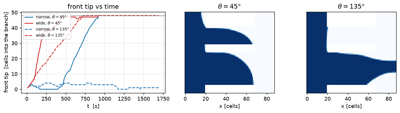
The number that matters is in the right-hand panels and in the S lines above: at \(\theta = 45°\) the narrow branch fills; at \(\theta = 135°\) it does not. Nothing but the contact angle changed.
Against Chatzis & Dullien
The same pair is now run at \(\mathrm{Ca} = 10^{-2}\) and \(10^{-4}\). The \(\mathrm{Ca} = 10^{-4}\) pair is the expensive one and it is capped at STEP_CAP = 12 000 steps — a full traverse there wants \(1.4\times10^{5}\), which is the arithmetic in “What this page cannot do” — so those two rows are reported as partial fills and their ordering, not their breakthrough times, is the result. Everything else is run to completion.
for ca in (1e-2, 1e-4):
    for th in (45.0, 135.0):
        DOUBLET[(th, ca)] = doublet(th, ca)
        report(DOUBLET[(th, ca)])
theta 45.0 Ca 1e-02 Re 100 |dPc|/dPmu 4.7
ran 528 of the 1381 steps a full traverse wants, to t = 74.6 s; capillary dt binds on 99 % of them
tip narrow 48/48 wide 47/48
S narrow 0.7143 wide 0.6217
breakthrough narrow 68.36183265221848, wide 74.59887130774439
pressure 63/400, max|div(open u)| 5.39e-09
theta 135.0 Ca 1e-02 Re 100 |dPc|/dPmu 4.7
ran 726 of the 1381 steps a full traverse wants, to t = 102.6 s; capillary dt binds on 99 % of them
tip narrow 47/48 wide 47/48
S narrow 0.9294 wide 0.8835
breakthrough narrow 101.09034914911513, wide 102.6496088129966
pressure 63/400, max|div(open u)| 1.48e-08
theta 45.0 Ca 1e-04 Re 1 |dPc|/dPmu 471.4
ran 12000 of the 138157 steps a full traverse wants, to t = 1701 s; capillary dt binds on 100 % of them
tip narrow 0/48 wide 25/48
S narrow 0.0000 wide 0.2419
breakthrough narrow None, wide None
pressure 86/400, max|div(open u)| 1.59e-09
theta 135.0 Ca 1e-04 Re 1 |dPc|/dPmu 471.4
ran 12000 of the 138157 steps a full traverse wants, to t = 1701 s; capillary dt binds on 100 % of them
tip narrow 3/48 wide 13/48
S narrow 0.0417 wide 0.2021
breakthrough narrow None, wide None
pressure 81/400, max|div(open u)| 1.10e-09def _bt(r, k):
return "—" if r["bt"][k] is None else f"{r['bt'][k]:.1f} s"
def _first(r):
"""Ordering on the TIP where both branches broke through, else on how far each got:
tip first, then the cross-section-mean front, then the branch saturation."""
n, w = r["bt"]["narrow"], r["bt"]["wide"]
if n is not None and w is not None:
return "narrow" if n < w else "wide"
if n is not None: return "narrow"
if w is not None: return "wide"
for k in (0, 1, 2):
a, b = r["f"]["narrow"][k], r["f"]["wide"][k]
if a != b:
return ("narrow" if a > b else "wide") + " *"
return "tied"
hdr = (f"{'Ca':>6} {'theta':>6} {'Re':>6} {'t_bt n':>9} {'t_bt w':>9} {'first':>7} "
f"{'tip n/w':>9} {'S_n':>7} {'S_w':>7} {'iters':>7} {'max|div|':>10}")
print(hdr); print("-" * len(hdr))
for ca in (1e-2, 1e-3, 1e-4):
for th in (45.0, 135.0):
r = DOUBLET[(th, ca)]
print(f"{ca:>6.0e} {th:>6.0f} {r['Re']:>6.3g} {_bt(r,'narrow'):>9} {_bt(r,'wide'):>9} "
f"{_first(r):>7} {r['f']['narrow'][0]:>4.0f}/{r['f']['wide'][0]:<4.0f} "
f"{r['f']['narrow'][2]:>7.4f} {r['f']['wide'][2]:>7.4f} "
f"{r['iters']:>3d}/{PRESS_CAP:<3d} {r['div']:>10.2e}")
npart = sum(1 for k, r in DOUBLET.items() if r["bt"]["narrow"] is None or r["bt"]["wide"] is None)
print(f"\n* = a PARTIAL fill: the branch ordering is read off the front position, not off a")
print(f" breakthrough time ({npart} of the 6 rows). Capped pressure solves: "
f"{sum(r['capped'] for r in DOUBLET.values())}.") Ca theta Re t_bt n t_bt w first tip n/w S_n S_w iters max|div|
---------------------------------------------------------------------------------------------
1e-02 45 100 68.4 s 74.6 s narrow 48/47 0.7143 0.6217 63/400 5.39e-09
1e-02 135 100 101.1 s 102.6 s narrow 47/47 0.9294 0.8835 63/400 1.48e-08
1e-03 45 10 921.4 s 453.6 s wide 47/48 0.7846 0.8448 119/400 1.45e-09
1e-03 135 10 — 708.8 s wide 1/48 0.0037 0.9117 98/400 4.37e-07
1e-04 45 1 — — wide * 0/25 0.0000 0.2419 86/400 1.59e-09
1e-04 135 1 — — wide * 3/13 0.0417 0.2021 81/400 1.10e-09
* = a PARTIAL fill: the branch ordering is read off the front position, not off a
breakthrough time (3 of the 6 rows). Capped pressure solves: 0.Note where the crossover should be: \(|\Delta P_c|/\Delta P_\mu\) is 4.7 even at the top of the sweep, so all three points are capillary-dominated and the classical criterion predicts narrow first at every \(\mathrm{Ca}\) for \(\theta = 45°\) and wide first at every \(\mathrm{Ca}\) for \(\theta = 135°\). The viscous-dominated regime for this geometry starts near \(\mathrm{Ca} \approx 5\times10^{-2}\).
Two readings, and they point in opposite directions:
- The drainage column is right, and at \(\mathrm{Ca} = 10^{-3}\) it is emphatic. The criterion asks for wide first at \(\theta = 135°\), and that is what the table gives at \(\mathrm{Ca} = 10^{-3}\) — the wide branch breaks through at 709 s, the narrow one never does, and they end at \(S = 0.004\) against \(0.912\): the non-wetting liquid gets one cell into the small pore and is held out of it while the wide branch takes the whole flux — and at \(10^{-4}\), where the wide front is four times the depth of the narrow one. At \(\mathrm{Ca} = 10^{-2}\) the two branches break through 1.6 s apart, which is exactly one sampling interval: that row is a tie, and it is reported as a tie. Set against the \(\theta = 45°\) run at the same \(\mathrm{Ca} = 10^{-3}\), the angle alone moves the narrow branch’s saturation by a factor of 200 — Equation 1 deciding, on its own, whether the small pore is filled or bypassed.
- The \(\theta = 45°\) column is right only at the top of the sweep, and the \(\mathrm{Ca}\) dependence runs backwards — and this is the page’s own finding, not a quoted one. Write the doublet’s flow split at a fixed total flux \(Q\): \[ Q_n = \frac{\Delta\Delta P_c + R_w Q}{R_n + R_w}, \tag{3}\] with \(R\) the viscous resistance of each branch’s liquid column. As \(Q\to0\) the wetting doublet must reach \(Q_n \to \Delta\Delta P_c/(R_n+R_w) > 0\) and hence \(Q_w < 0\): the narrow branch imbibes while drawing liquid back out of the wide one. That limit needs the contact line to advance under its own suction. The measured ordering flips between \(\mathrm{Ca} = 10^{-3}\) and \(10^{-2}\), i.e. where the imposed velocity crosses a numerical mobility of the contact line, not at the physical Chatzis–Dullien crossover. The imbibition half of this page is therefore a finding about the solver, not about the doublet, and the next cell says which part of the solver.
2. Imbibition into a sphere packing
36 grains are dropped into a laterally periodic column and settled with a soft-sphere relaxation written in NumPy, so the scene has no dependency on the dem package. The SDF grain radius is \(0.85\) of the contact radius — grains that touch leave throats the grid cannot resolve, and shrinking them is the standard device (the bubble through a packing page uses the same factor).
PNX, PNY, PNZ = 48, 48, 96
Z_BED, N_GRAIN, R_CONTACT, F_SDF = 16.0, 36, 8.0, 0.85
R_SDF = F_SDF * R_CONTACT

def settle(n=N_GRAIN, L=float(PNX), R=R_CONTACT, seed=7, iters=4000, dz=0.02):
    rng = np.random.default_rng(seed)
    P = np.zeros((n, 3))
    P[:, :2] = rng.uniform(0.0, L, (n, 2))
    P[:, 2] = R + 2.1 * R * (np.arange(n) // 6) + rng.uniform(-0.4, 0.4, n)
    for _ in range(iters):
        P[:, 2] -= dz
        for _ in range(4):
            d = P[None, :, :] - P[:, None, :]
            d[:, :, 0] -= L * np.round(d[:, :, 0] / L)
            d[:, :, 1] -= L * np.round(d[:, :, 1] / L)
            r = np.sqrt((d ** 2).sum(-1)); np.fill_diagonal(r, 1e9)
            ov = np.maximum(2.0 * R - r, 0.0)
            u = d / np.maximum(r, 1e-9)[:, :, None]
            P -= 0.5 * (ov[:, :, None] * u).sum(axis=1)
            P[:, 2] = np.maximum(P[:, 2], R)
        P[:, :2] %= L
    return P

def bed_sdf(P, Rg=R_SDF, z0=Z_BED):
    L = float(PNX); Q = P.copy(); Q[:, 2] += z0 - R_CONTACT
    g = np.arange(PNX) + 0.5
    X, Y, Z = np.meshgrid(g, np.arange(PNY) + 0.5, np.arange(PNZ) + 0.5, indexing="ij")
    phi = np.full((PNX, PNY, PNZ), 1e30)
    for k in range(len(Q)):
        dx = X - Q[k, 0]; dx -= L * np.round(dx / L)
        dy = Y - Q[k, 1]; dy -= L * np.round(dy / L)
        phi = np.minimum(phi, np.sqrt(dx * dx + dy * dy + (Z - Q[k, 2]) ** 2) - Rg)
    return np.asfortranarray(phi)

CENTRES = settle()
SDF_P = bed_sdf(CENTRES)
BOT = Z_BED + CENTRES[:, 2].min() - R_CONTACT
TOP = Z_BED + CENTRES[:, 2].max() - R_CONTACT + R_SDF
KLO, KHI = int(math.ceil(BOT + R_SDF)), int(math.floor(TOP - R_SDF))
POROSITY = float((SDF_P[:, :, KLO:KHI] > 0).mean())
print(f"bed surfaces span z = {BOT:.1f} .. {TOP:.1f} "
      f"({(TOP-BOT)/(2*R_SDF):.1f} SDF grain diameters); core z = {KLO} .. {KHI}")
print(f"porosity over the bed core: {POROSITY:.4f}")
print(f"inlet plenum z = 0 .. {int(BOT)}, outlet plenum z = {int(TOP)} .. {PNZ}: "
      f"the solid is clear of both open faces")
bed surfaces span z = 16.0 .. 67.0 (3.7 SDF grain diameters); core z = 23 .. 60
porosity over the bed core: 0.6023
inlet plenum z = 0 .. 16, outlet plenum z = 66 .. 96: the solid is clear of both open facesOne number about this bed is worth having before the results. The percolation throat radius — the max–min path of the SDF from the bottom of the bed to the top, i.e. the widest bottleneck a front must squeeze through — was measured on this scene at about 2.2 cells by a Dijkstra max–min sweep. That is at or below the \(\approx2.5\)-cell floor where the curvature scheme’s height-function cascade is permanently in its PLIC-volumetric fallback, so the bottleneck’s meniscus is represented but not resolved. It is one more reason to read this case as a wettability contrast rather than as a saturation measurement.
from scipy import ndimage

def trapped_gas(C, eps, klo, khi):
    """Fraction of the bed pore volume held as gas NOT connected to the outlet plenum."""
    gas = (C < 0.5) & (eps > 0.0)
    lab, nlab = ndimage.label(gas)
    parent = list(range(nlab + 1))
    def find(x):
        while parent[x] != x:
            parent[x] = parent[parent[x]]; x = parent[x]
        return x
    for a, b in ((lab[0], lab[-1]), (lab[:, 0], lab[:, -1])):     # periodic x and y seams
        m = (a > 0) & (b > 0)
        for u, v in zip(a[m].ravel().tolist(), b[m].ravel().tolist()):
            ru, rv = find(u), find(v)
            if ru != rv:
                parent[max(ru, rv)] = min(ru, rv)
    lab = np.array([find(i) if i else 0 for i in range(nlab + 1)])[lab]
    openr = list(set(np.unique(lab[:, :, khi:]).tolist()) - {0})
    bed = slice(klo, khi)
    pore = float(eps[:, :, bed].sum())
    sel = gas[:, :, bed] & ~np.isin(lab[:, :, bed], openr)
    return float((eps[:, :, bed] * (1.0 - C[:, :, bed]) * sel).sum()) / pore

def packing(theta_deg, ca=1e-3, step_cap=STEP_CAP, after=0.25, every=100):
    U = ca * SIGMA / MU_L
    s = flow.Solver(PNX, PNY, PNZ)
    s.set_rho(RHO_L); s.set_mu(MU_L); s.set_dt(0.05)
    s.set_domain_bc(4, 2, 0.0, 0.0, U)          # -z inflow (liquid), x/y periodic
    s.set_domain_bc(5, 3, 0.0, 0.0, 0.0)        # +z outflow
    s.set_velocity_solver_params(20)
    s.set_pressure_multigrid(True, levels=5)
    s.set_pressure_solver_params(80)
    s.set_solid(SDF_P, cutcell_pressure=True)
    s.enable_vof()
    c0 = np.zeros((PNX, PNY, PNZ), order="F"); c0[:, :, :KLO - 2] = 1.0
    s.set_vof(c0)
    s.set_property_model("rho", "linear", "C", [RHO_G, RHO_L - RHO_G])
    s.set_property_model("mu",  "linear", "C", [MU_G,  MU_L  - MU_G])
    s.enable_vof_momentum(RHO_G, RHO_L)
    s.set_surface_tension(SIGMA); s.set_capillary_cfl(CAP_CFL)
    s.set_contact_angle(theta_deg)
    s.set_pressure_fcg(True, PRESS_CAP, 1e-8)
    s.set_vof_inflow(4, 1.0); s.set_vof_backflow(5, 0.0)

    eps = np.asarray(s.vof_geometry(0))
    pore = float(eps[:, :, KLO:KHI].sum())
    h, hist, bt, t, n, stop, err = Health(), [], None, 0.0, 0, None, None
    ncfl, t0 = 0, time.time()
    for _ in range(step_cap):
        L = s.vof_step_limits()
        dtc = CAP_CFL * L["capillary_dt"]
        dt = min(dtc, 0.8 * L["cfl_dt"]) if L["cfl_dt"] > 0 else dtc
        ncfl += int(dt < 0.999 * dtc)
        s.set_dt(dt)
        try:
            s.step()
        except RuntimeError as exc:
            err = str(exc); break
        t += dt; n += 1
        h.sample(s)
        if n % every == 0:
            C = np.asarray(s.get_vof())
            S = float((C[:, :, KLO:KHI] * eps[:, :, KLO:KHI]).sum() / pore)
            hist.append((t, S))
            if bt is None and float((C[:, :, KHI - 1] * eps[:, :, KHI - 1]).max()) > 0.5:
                bt = (t, S); stop = n + int(after * n)
            if stop is not None and n >= stop:
                break
    C = np.asarray(s.get_vof())
    S = float((C[:, :, KLO:KHI] * eps[:, :, KLO:KHI]).sum() / pore)
    return dict(theta=theta_deg, t=t, n=n, ms=1000 * (time.time() - t0) / max(n, 1),
                hist=np.array(hist), bt=bt, S=S, err=err, cfl_frac=ncfl / max(n, 1),
                trapped=trapped_gas(C, eps, KLO, KHI), C=C, eps=eps,
                iters=h.iters, capped=h.capped, div=h.div)

PACK = {}
for th in (30.0, 60.0):
    r = packing(th)
    PACK[th] = r
    if r["bt"] is None:
        print(f"theta {th:5.1f}: NO breakthrough inside {r['n']} steps (t = {r['t']:.4g} s)")
    else:
        print(f"theta {th:5.1f}: breakthrough at t = {r['bt'][0]:.4g} s with bed saturation "
              f"{r['bt'][1]:.4f}; final S = {r['S']:.4f}, trapped gas {r['trapped']:.4f}")
    print(f"   {r['n']} steps, capillary dt binds on {100*(1-r['cfl_frac']):.0f} % of them; "
          f"pressure {r['iters']}/{PRESS_CAP}"
          f"{'' if not r['capped'] else ' *** CAPPED -> INVALID ***'}, max|div| {r['div']:.2e}"
          + ("" if r["err"] is None else f"\n   STOPPED BY: {r['err']}"))
BT = {th: (PACK[th]["bt"] or (float("nan"), float("nan"))) for th in PACK}
theta 30.0: breakthrough at t = 800.5 s with bed saturation 0.8255; final S = 0.9826, trapped gas 0.0117
9300 steps, capillary dt binds on 24 % of them; pressure 30/400, max|div| 5.05e-06
theta 60.0: breakthrough at t = 809.1 s with bed saturation 0.8350; final S = 0.9736, trapped gas 0.0113
7800 steps, capillary dt binds on 65 % of them; pressure 30/400, max|div| 1.59e-06fig, ax = plt.subplots(1, 3, figsize=(11, 3.1),
gridspec_kw={"width_ratios": [1.25, 1, 1]})
for th, col in ((30.0, BLUE), (60.0, ORANGE)):
r = PACK[th]
if r["hist"].ndim == 2:
ax[0].plot(r["hist"][:, 0], r["hist"][:, 1], color=col, label=f"$\\theta={th:.0f}°$")
if r["bt"] is not None:
ax[0].plot([r["bt"][0]], [r["bt"][1]], "o", color=col, ms=5)
ax[0].set_xlabel("t [s]"); ax[0].set_ylabel("bed liquid saturation $S$")
ax[0].legend(fontsize=8); ax[0].set_title("saturation vs time (dots: breakthrough)")
for k, th in enumerate((30.0, 60.0)):
r = PACK[th]
j = PNY // 2
img = np.where(r["eps"][:, j, :] <= 0.0, np.nan, r["C"][:, j, :])
a = ax[k + 1]
a.imshow(np.ones_like(img.T), origin="lower", cmap="gray", vmin=0, vmax=1)
a.imshow(img.T, origin="lower", cmap="Blues", vmin=0, vmax=1)
a.set_title(f"$\\theta = {th:.0f}°$"); a.set_xlabel("x [cells]")
a.set_yticks([]); a.grid(False)
plt.tight_layout()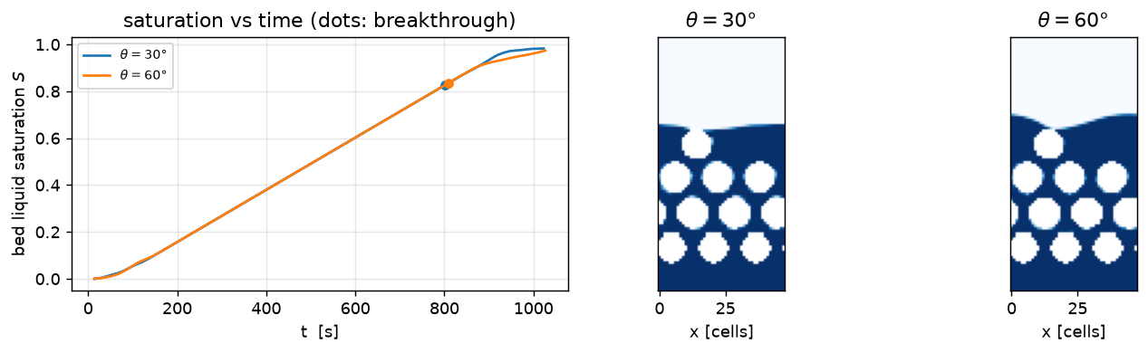
The bed is invaded nearly completely at both angles — final \(S\) of 0.98 and 0.97 — and the trapped gas is of order a per cent of the pore volume in both (0.012 against 0.011): at this capillary number and this small a bed the trapping is set by the geometry, not by the angle.
The quantity that carries the physics is the saturation at breakthrough: a flat, compact front only reaches the top of the bed once most of the pore space behind it is full, while a fingered one arrives early and dry. Strong imbibition is supposed to produce the first and weak imbibition the second, so halving the contact angle ought to move this number a long way.
It does not move it at all. The strongly wetting bed breaks through at 800.5 s at a bed saturation of 0.825, the weakly wetting one at 809.1 s at 0.835 — a difference of 1 % in the saturation and 1 % in the time, against a factor-of-two change in \(\cos\theta\). The trapped gas agrees to the third digit as well.
The wettability effect the textbook predicts is not there. Its sign, in as far as a one-per-cent difference has one, is the inverted one — the more wetting bed is marginally the earlier and the drier — which is the same direction as the doublet’s \(\theta = 45°\) column. The mechanism is the one §1’s slip control isolated: with the contact line’s mobility set by a resistance in the wetting band that neither the angle nor the wall condition controls, a lower \(\theta\) cannot fill behind the front any faster. What it does buy is extra capillary suction into the throats the front has already reached, which accelerates the leading fingers rather than filling in behind them — and here that buys almost nothing.
3. A micromodel: wettability and the invasion pattern
Zhao, MacMinn & Juanes (Zhao et al. 2016) took a disordered array of posts and showed that wettability alone moves the displacement pattern from compact (strong imbibition) to fingered (drainage); the same geometry later became the benchmark on which eleven pore-scale codes were compared side by side (Zhao et al. 2019). The array here is a jittered staggered lattice of 30 posts in \(128\times128\times4\) cells, invaded at three angles.
WarningPost count, porosity and grid: pick two
The obvious array — around 60 posts at a porosity of 0.6 — was tried first and does not survive, and the measurement is worth stating rather than hiding. A square array at porosity 0.6 has throats of \(0.286\times\) the lattice spacing, which at 56 posts on this grid is 3.1 cells. That configuration ran to 0.12 pore volumes injected and then emitted CutcellMG::solveFCG: preconditioner produced non-finite z, with \(\max|u|\) at 93 times the inlet velocity. The array below keeps the disorder and the geometry class but trades post count for throat width: 30 posts, narrowest throat 6.4 cells, porosity \(\approx0.71\).
Two candidate mechanisms, and this page does not separate them: (a) the contact-angle fill writes a three-cell band into the solid on each side of a throat, so at 3.1 cells the two posts’ bands meet in the middle of it — the same overlap that made the solver’s own four-cell-plate capillary-rise test inconclusive; (b) a Haines jump through a throat whose meniscus radius is \(\approx1.5\) cells is simply unresolved. Local velocities in a real pore-filling event run up towards the capillary velocity \(\sigma/\mu_\ell = 25\), a thousand times the inlet velocity here, so a \(\max|u|\) far above the superficial one is expected physics and only its resolution is in question.
MNX, MNY, MNZ = 128, 128, 4
NCOL, NROW, X0, DX = 5, 6, 20.0, 21.5
DY, R_POST, JITTER, MIN_GAP = MNY / NROW, 6.5, 1.5, 6.0
X_IN, X_BT = 10.0, 118.0

def posts(seed=3):
    rng = np.random.default_rng(seed)
    base = np.array([(X0 + i * DX, (j + 0.5 * (i % 2)) * DY)
                     for i in range(NCOL) for j in range(NROW)])
    for _ in range(20000):
        P = base + rng.uniform(-JITTER, JITTER, base.shape); P[:, 1] %= MNY
        d = P[None, :, :] - P[:, None, :]
        d[:, :, 1] -= MNY * np.round(d[:, :, 1] / MNY)
        r = np.sqrt((d ** 2).sum(-1)); np.fill_diagonal(r, 1e9)
        if (r - 2 * R_POST).min() >= MIN_GAP:
            return P, float((r - 2 * R_POST).min())
    raise RuntimeError("no admissible lattice")

def post_sdf(P):
    x = (np.arange(MNX) + 0.5)[:, None]; y = (np.arange(MNY) + 0.5)[None, :]
    phi = np.full((MNX, MNY), 1e30)
    for cx, cy in P:
        dy = y - cy; dy -= MNY * np.round(dy / MNY)
        phi = np.minimum(phi, np.sqrt((x - cx) ** 2 + dy ** 2) - R_POST)
    return np.asfortranarray(np.broadcast_to(phi[:, :, None], (MNX, MNY, MNZ)).astype(float).copy())

POSTS, GAP = posts()
SDF_M = post_sdf(POSTS)
POR_M = float((SDF_M[int(X_IN):int(X_BT), :, 0] > 0).mean())
print(f"{len(POSTS)} posts of radius {R_POST}; porosity {POR_M:.4f}; "
      f"narrowest throat {GAP:.2f} cells")
30 posts of radius 6.5; porosity 0.7123; narrowest throat 6.38 cells
WarningCorner films are not represented, and this is the case that needs them
The standing warning about this benchmark is that corner films decide imbibition fidelity — the strong-imbibition end of Zhao’s experiment is carried by liquid running ahead in the corners between the posts and the confining plates, and that is what defeated most of the codes in the 2019 comparison. A quasi-2D slab four cells thick has no such corner to resolve, and this scheme has no sub-grid film model. Read the trend below, not the saturations.
def box_dimension(mask, sizes=(1, 2, 4, 8, 16, 32)):
    nx, ny = mask.shape; pts = []
    for e in sizes:
        mx, my = (nx // e) * e, (ny // e) * e
        blk = mask[:mx, :my].reshape(mx // e, e, my // e, e).any(axis=(1, 3))
        if blk.sum():
            pts.append((e, int(blk.sum())))
    if len(pts) < 2:                       # nothing invaded yet: no slope to fit
        return float("nan"), pts
    x = np.log([1.0 / p[0] for p in pts]); y = np.log([float(p[1]) for p in pts])
    return float(np.polyfit(x, y, 1)[0]), pts

def front_stats(inv):
    """Roughness of the invasion front — the discriminator Zhao's experiment is really about.
    For every transverse row the liquid reached, the front is the furthest x it reached; a COMPACT
    displacement reaches every row with a small standard deviation, a FINGERED one has a large one,
    a deep maximum, and leaves rows untouched."""
    reach = np.array([np.max(np.nonzero(inv[:, j])[0]) if inv[:, j].any() else -1
                      for j in range(inv.shape[1])])
    ok = reach >= 0
    lab, n = ndimage.label(inv)
    nan = float("nan")
    return dict(rows=int(ok.sum()), nrows=int(inv.shape[1]),
                mean=float(reach[ok].mean()) if ok.any() else nan,
                std=float(reach[ok].std()) if ok.any() else nan,
                max=int(reach.max()), clusters=int(n))


def micromodel(theta_deg, ca=1e-3, pv_stop=0.10, step_cap=STEP_CAP, every=60):
    U = ca * SIGMA / MU_L
    s = flow.Solver(MNX, MNY, MNZ)
    s.set_rho(RHO_L); s.set_mu(MU_L); s.set_dt(0.05)
    s.set_domain_bc(0, 2, U, 0.0, 0.0); s.set_domain_bc(1, 3, 0.0, 0.0, 0.0)
    s.set_velocity_solver_params(20)
    s.set_pressure_multigrid(True, levels=5); s.set_pressure_solver_params(80)
    s.set_solid(SDF_M, cutcell_pressure=True)
    s.enable_vof()
    c0 = np.zeros((MNX, MNY, MNZ), order="F"); c0[: int(X_IN), :, :] = 1.0
    s.set_vof(c0)
    s.set_property_model("rho", "linear", "C", [RHO_G, RHO_L - RHO_G])
    s.set_property_model("mu",  "linear", "C", [MU_G,  MU_L  - MU_G])
    s.enable_vof_momentum(RHO_G, RHO_L)
    s.set_surface_tension(SIGMA); s.set_capillary_cfl(CAP_CFL)
    s.set_contact_angle(theta_deg)
    s.set_pressure_fcg(True, PRESS_CAP, 1e-8)
    s.set_vof_inflow(0, 1.0); s.set_vof_backflow(1, 0.0)

    eps = np.asarray(s.vof_geometry(0)); arr = slice(int(X_IN), int(X_BT))
    pore = float(eps[arr].sum())
    h, hist, t, n, bt, err = Health(), [], 0.0, 0, None, None
    ncfl, t0 = 0, time.time()
    for _ in range(step_cap):
        L = s.vof_step_limits()
        dtc = CAP_CFL * L["capillary_dt"]
        dt = min(dtc, 0.8 * L["cfl_dt"]) if L["cfl_dt"] > 0 else dtc
        ncfl += int(dt < 0.999 * dtc)
        s.set_dt(dt)
        try:
            s.step()
        except RuntimeError as exc:
            err = str(exc); break
        t += dt; n += 1
        h.sample(s)
        if n % every == 0:
            C = np.asarray(s.get_vof())
            S = float((C[arr] * eps[arr]).sum() / pore)
            pv = U * MNY * MNZ * t / pore
            hist.append((t, pv, S))
            if float(C[int(X_BT) - 1, :, :].max()) > 0.5:
                bt = (t, pv, S); break
            if pv >= pv_stop:
                break
    C = np.asarray(s.get_vof())
    mid = MNZ // 2
    inv = (C[:, :, mid] > 0.5) & (eps[:, :, mid] > 0.0)
    D, pts = box_dimension(inv[arr])
    fs = front_stats(inv[arr])
    return dict(theta=theta_deg, t=t, n=n, ms=1000 * (time.time() - t0) / max(n, 1),
                hist=np.array(hist), bt=bt, D=D, boxes=pts, front=fs, err=err,
                cfl_frac=ncfl / max(n, 1),
                S=float((C[arr] * eps[arr]).sum() / pore),
                pv=U * MNY * MNZ * t / pore, inv=inv, eps=eps[:, :, mid],
                iters=h.iters, capped=h.capped, div=h.div)

MICRO = {}
for th in (45.0, 90.0, 135.0):
    r = micromodel(th)
    MICRO[th] = r
    f = r["front"]
    tag = "breakthrough" if r["bt"] else "stopped at a common injected volume"
    print(f"theta {th:5.1f}: {tag}; injected {r['pv']:.3f} PV, array saturation "
          f"{r['S']:.4f}, box dimension D = {r['D']:.3f}")
    print(f"   front: reached {f['rows']}/{f['nrows']} rows, mean {f['mean']:.2f} cells, "
          f"std {f['std']:.2f}, deepest finger {f['max']}, {f['clusters']} cluster(s)")
    print(f"   {r['n']} steps, Weymouth-Yue cap binds on {100*r['cfl_frac']:.0f} % of them; "
          f"pressure {r['iters']}/{PRESS_CAP}"
          f"{'' if not r['capped'] else ' *** CAPPED -> INVALID ***'}, max|div| {r['div']:.2e}"
          + ("" if r["err"] is None else f"\n   STOPPED BY: {r['err']}"))
theta 45.0: stopped at a common injected volume; injected 0.102 PV, array saturation 0.1024, box dimension D = 1.624
front: reached 128/128 rows, mean 7.48 cells, std 5.06, deepest finger 18, 1 cluster(s)
2340 steps, Weymouth-Yue cap binds on 11 % of them; pressure 130/400, max|div| 1.51e-06
theta 90.0: stopped at a common injected volume; injected 0.102 PV, array saturation 0.1021, box dimension D = 1.605
front: reached 128/128 rows, mean 7.34 cells, std 5.11, deepest finger 17, 1 cluster(s)
2220 steps, Weymouth-Yue cap binds on 0 % of them; pressure 179/400, max|div| 7.10e-09
theta 135.0: stopped at a common injected volume; injected 0.102 PV, array saturation 0.1021, box dimension D = 1.636
front: reached 128/128 rows, mean 7.11 cells, std 4.55, deepest finger 15, 1 cluster(s)
2220 steps, Weymouth-Yue cap binds on 0 % of them; pressure 170/400, max|div| 1.54e-09fig, ax = plt.subplots(1, 3, figsize=(11, 3.6))
for k, th in enumerate((45.0, 90.0, 135.0)):
r = MICRO[th]
img = np.where(r["eps"] <= 0.0, np.nan, r["inv"].astype(float))
a = ax[k]
a.imshow(np.ones_like(img.T), origin="lower", cmap="gray", vmin=0, vmax=1)
a.imshow(img.T, origin="lower", cmap="Blues", vmin=0, vmax=1)
a.set_title(f"$\\theta = {th:.0f}°$ $D = {r['D']:.2f}$ front std "
f"{r['front']['std']:.1f}")
a.set_xlabel("x [cells]"); a.set_yticks([]); a.grid(False)
plt.tight_layout()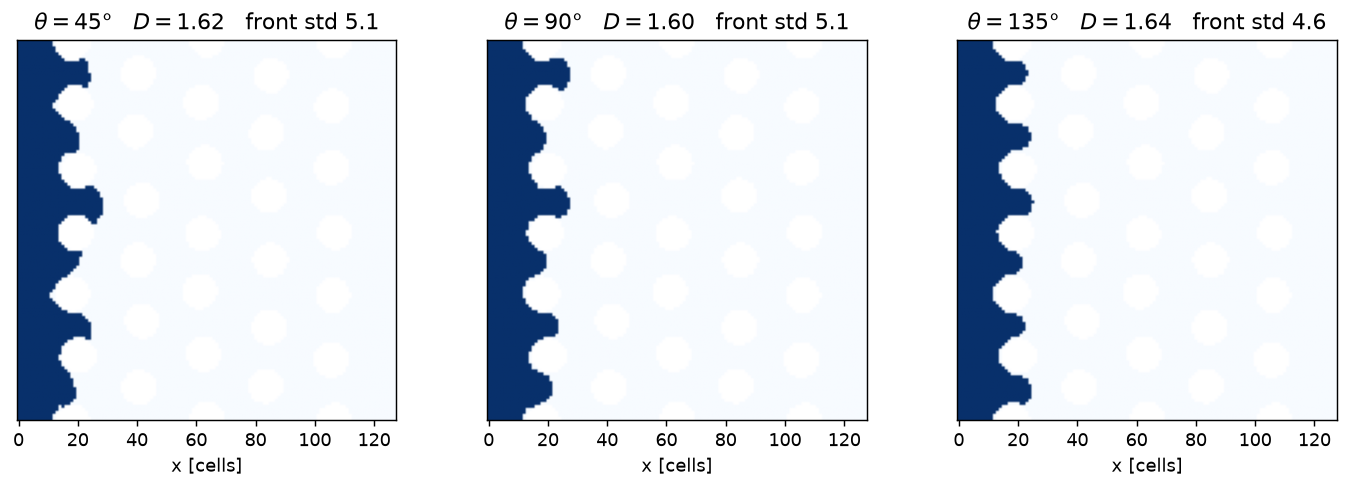
At a common injected volume the saturation is equal by construction, so it carries no information; the discriminators are the box dimension and the roughness of the front.
hdr = (f"{'theta':>6} {'PV':>7} {'S':>7} {'D_box':>7} {'rows':>9} {'mean':>7} "
       f"{'std':>7} {'deepest':>8} {'clusters':>9} {'iters':>8} {'max|div|':>10}")
print(hdr); print("-" * len(hdr))
for th in (45.0, 90.0, 135.0):
    r = MICRO[th]; f = r["front"]
    print(f"{th:>6.0f} {r['pv']:>7.4f} {r['S']:>7.4f} {r['D']:>7.3f} "
          f"{f['rows']:>4d}/{f['nrows']:<4d} {f['mean']:>7.2f} {f['std']:>7.2f} "
          f"{f['max']:>8d} {f['clusters']:>9d} {r['iters']:>4d}/{PRESS_CAP:<3d} {r['div']:>10.2e}")
theta PV S D_box rows mean std deepest clusters iters max|div|
-----------------------------------------------------------------------------------------------
45 0.1025 0.1024 1.624 128/128 7.48 5.06 18 1 130/400 1.51e-06
90 0.1021 0.1021 1.605 128/128 7.34 5.11 17 1 179/400 7.10e-09
135 0.1022 0.1021 1.636 128/128 7.11 4.55 15 1 170/400 1.54e-09The published trend is not reproduced — neither its size nor, in as far as it has one here, its sign. Zhao’s result is that strong imbibition displaces compactly (cooperative pore filling) and drainage fingers, and that the two are unmistakably different to the eye. Measured here at a common injected volume, the entire spread over \(90°\) of contact angle is this: the front’s standard deviation goes 5.06 / 5.11 / 4.55 cells, the deepest finger 18 / 17 / 15, and the box dimension 1.624 / 1.605 / 1.636 — not ordered in \(\theta\) at all. Every angle reaches every one of the 128 transverse rows, as a single connected cluster. The three panels above are, to the eye, the same displacement.
Two things can still be said, and they are worth more than the non-result. The wetting extreme is the rougher of the two, by 11 % and with the deeper finger, so what little dependence exists runs backwards against the experiment. And the ordering is broken by the neutral case, which sits at the rough end alongside the wetting one — which is what a pattern set by the imposed flux and the array’s own disorder, rather than by wettability, looks like.
This is the third case on this page to come out the same way, and it is the one where the mechanism is easiest to name: cooperative pore filling requires the contact line to run ahead along the post walls, and §1’s slip control shows that what forbids that motion is not the wall’s velocity condition — turning on an explicit Navier slip does not restore it — but a resistance local to the wetting band. With the line effectively pinned the imposed angle can no longer choose which pore fills next; the flux and the geometry do, and they do it the same way at every \(\theta\). What the angle still buys is extra suction at the menisci already at the front, which accelerates whichever finger is furthest — the wrong sign for a compact displacement, and the reason the wetting case is the rougher one.
Two health notes, recorded rather than smoothed. First, the \(\theta = 45°\) run is the violent one on its own diagnostics — its max_open_divergence_projected() and its share of steps on the Weymouth–Yue cap are both the worst of the three in the table above, consistently with the fingering. Second, the trajectory is chaotic: the same scene run with 12 OpenMP threads instead of 4 was measured reaching \(\max|u| = 4.12\) where the 4-thread run read \(0.632\) at the same step, because the reduction order differs at \(10^{-16}\) and invasion percolation in a disordered array amplifies it. The pattern statistics are the reportable quantity here; a trajectory is not — and a re-execution of this page on different hardware will not reproduce the fields cell for cell.
What this page cannot do
Five limits, each measured rather than guessed:
- The contact line’s mobility is set by the wetting band, and nothing on the API controls it. The two pieces a reader would reach for both exist and both are exact on their own tests — the apparent angle of a moving line is a Cox–Voinov function of its speed (
set_contact_angle_dynamic), and the wall’s tangential momentum condition is a true Navier condition (set_wall_slip_length, exercised in §1). Neither is the limiter. Capillary rise runs \(175\times\) slower than Lucas–Washburn, the slip recovers \(26\,\%\) of that, and the missing resistance is independent of the channel width (the rise speed goes as \(1/w\) where the law says \(w\)) — i.e. it is local to the few-cell band at the wall, not to the confinement. Everything on this page that depends on a wetting front advancing under its own suction is qualitative, and the three cases below either fail in that direction or show no wettability dependence where a large one is expected. - No corner films. Named in the VoF plan as the thing that defeated most 2019-era codes on exactly this micromodel benchmark — and the strong-imbibition end of Zhao’s experiment is carried by them.
- Density ratio 100, not 1000. The momentum-consistent transport’s own uniform-velocity identity is floored at \(10^{-7}\) by the solver’s float momentum-operator storage, and a resting pool at ratio 1000 was measured to pick up \(3\times10^{-2}\) of the driving velocity. Ratio 100 is the rated regime.
- The capillary time step usually — not always — sets the cost. In the low-\(\mathrm{Ca}\) runs above the Brackbill limit binds on nearly every step; at \(\mathrm{Ca}=10^{-2}\), and inside the packing where a throat manufactures a local jet, the Weymouth–Yue advective cap takes over for most of the run. Both limits are therefore re-picked from
vof_step_limits()every step. The arithmetic is not tuning: \(\Delta t_\sigma \sim h^{3/2}\) against \(\Delta t_{\text{CFL}} \sim h\), so refinement makes it worse. - Two runs are budgeted, not completed. Eliminating the fluid properties in favour of the two dimensionless groups, the number of steps to move a front a distance \(L\) through a channel of width \(w\) is \(N \sim L\sqrt{w/(\mathrm{Re}\, \mathrm{Ca})}\) — independent of \(\sigma\), \(\rho\) and \(\mu\) separately. There is no choice of fluids that makes a pore-scale VoF run cheaper at a given geometry, Reynolds and capillary number; the only levers are a shorter path, a larger \(\mathrm{Re}\), or a larger \(\mathrm{Ca}\). That is why the \(\mathrm{Ca}=10^{-4}\) doublet rows are capped at 12 000 of the \(1.4\times10^{5}\) steps a full traverse wants and are reported as partial fills, and why the micromodel is compared at a common injected volume instead of at breakthrough.
Adapt this yourself
- Change the width ratio.
W_NARROW/W_WIDEare the doublet’s only geometric knobs that matter; Equation 1 and Equation 2 both scale with them, so the crossover capillary number moves as \(w^{-1}\) against \(L\,w^{-2}\). - Move the crossover into range. \(|\Delta P_c|/\Delta P_\mu\) is printed for every run; lengthening
BRANCHraises \(\Delta P_\mu\) linearly and is the cheapest way to reach the viscous-dominated regime without raising the Reynolds number. - Drain instead of imbibe. Swap the initial colour and the inflow datum (
set_vof_inflow(face, 0.0)with a liquid-filled domain) to push gas into a saturated packing — that is the bubble through a packing page’s problem in a driven column. - Use a real bed.
settlehere is a NumPy toy; swap it fordem’s packing as the bubble page does, and nothing on the fluid side changes. - Turn the wall slip up.
set_wall_slip_length(λ)is one line and costs nothing atλ = 0; §1 sweeps it over a factor of five on the doublet. It is worth running on your own geometry before concluding that a wetting result is physics — a result that moves a lot with λ is being set by the wall model, and one that does not (like this page’s) is being set by something else. - Go multi-rank. All of it runs under
mpirun -np N python …: the colour halo, the wetting band fill and the cut-cell fluxes are all decomposition-independent by construction.
Reproduce this
The compiled solver runs this page, so its outputs are frozen into the site. The full campaign (three capillary numbers on the doublet, both packing angles, three micromodel angles, with every number printed) lives in the flow repository as three standalone scripts:
cd flow && source ../.venv/bin/activate
export PYTHONPATH=$PWD/build_cuda
python tests/study/pore_scale/pore_doublet.py       --theta 45,135 --ca 1e-4,1e-3,1e-2
python tests/study/pore_scale/imbibition_packing.py --theta 30,60  --ca 1e-3
python tests/study/pore_scale/micromodel_2d.py      --theta 45,90,135 --ca 1e-3
# --quick shortens every run to a few hundred steps (shape, not physics);
# --slip <lambda cells> is the Navier-slip control of section 1.
python tests/study/pore_scale/pore_doublet.py --theta 45 --ca 1e-3 --slip 0.5
To regenerate this page:
pip install peclet            # the solver, from PyPI
quarto render examples/pore-scale-imbibition/index.qmd --execute
# ...or against a local source build of the suite (GPU):
PECLET_LOCAL_BUILD=/path/to/suite/flow/build_cuda OMP_NUM_THREADS=8 OMP_PROC_BIND=false \
  quarto render examples/pore-scale-imbibition/index.qmd --execute
References
Cited above, and rendered from the gallery’s shared references.bib. The Weymouth–Yue geometric transport (Weymouth and Yue 2010), the balanced-force surface tension (Brackbill et al. 1992), the height-function contact angle (Afkhami and Bussmann 2008) and the variable-density outflow operator (Rusche 2002) are the solver pieces this page composes; the physics it is measured against is the pore doublet (Chatzis and Dullien 1983), the micromodel (Zhao et al. 2016, 2019) and capillary rise (Lucas 1918; Washburn 1921).
Afkhami, S., and M. Bussmann. 2008. “Height Functions for Applying Contact Angles to 2D VOF Simulations.” International Journal for Numerical Methods in Fluids 57 (4): 453–72. https://doi.org/10.1002/fld.1651.
Brackbill, J. U., D. B. Kothe, and C. Zemach. 1992. “A Continuum Method for Modeling Surface Tension.” Journal of Computational Physics 100 (2): 335–54. https://doi.org/10.1016/0021-9991(92)90240-Y.
Chatzis, I., and F. A. L. Dullien. 1983. “Dynamic Immiscible Displacement Mechanisms in Pore Doublets: Theory Versus Experiment.” Journal of Colloid and Interface Science 91 (1): 199–222. https://doi.org/10.1016/0021-9797(83)90326-0.
Lucas, Richard. 1918. “Ueber Das Zeitgesetz Des Kapillaren Aufstiegs von Flüssigkeiten.” Kolloid-Zeitschrift 23: 15–22. https://doi.org/10.1007/BF01461107.
Rusche, Henrik. 2002. “Computational Fluid Dynamics of Dispersed Two-Phase Flows at High Phase Fractions.” PhD thesis, Imperial College London.
Washburn, Edward W. 1921. “The Dynamics of Capillary Flow.” Physical Review 17 (3): 273–83. https://doi.org/10.1103/PhysRev.17.273.
Weymouth, G. D., and Dick K.-P. Yue. 2010. “Conservative Volume-of-Fluid Method for Free-Surface Simulations on Cartesian-Grids.” Journal of Computational Physics 229 (8): 2853–65. https://doi.org/10.1016/j.jcp.2009.12.018.
Zhao, Benzhong, Christopher W. MacMinn, and Ruben Juanes. 2016. “Wettability Control on Multiphase Flow in Patterned Microfluidics.” Proceedings of the National Academy of Sciences 113 (37): 10251–56. https://doi.org/10.1073/pnas.1603387113.
Zhao, Benzhong, Christopher W. MacMinn, Bauyrzhan K. Primkulov, et al. 2019. “Comprehensive Comparison of Pore-Scale Models for Multiphase Flow in Porous Media.” Proceedings of the National Academy of Sciences 116 (28): 13799–806. https://doi.org/10.1073/pnas.1901619116.