import importlib.util, os, subprocess, sys
_local = os.environ.get("PECLET_LOCAL_BUILD")
if _local:
    for p in _local.split(os.pathsep):
        sys.path.insert(0, p)
elif importlib.util.find_spec("peclet") is None:
    # peclet-coupling is sdist-only (it builds its Kokkos kernels from source against a Kokkos prefix);
    # on a plain runtime install the CPU family + the coupling extra.
subprocess.run([sys.executable, "-m", "pip", "install", "-q", "peclet[cfd-dem]"], check=True)Gas–solid fluidized bed: online CFD–DEM coupling
Blow gas up through a cylinder of grains until the bed unpacks and boils — the two solvers exchanging drag and void fraction every step — then reproduce a million-particle X-ray tomography benchmark, bubble by bubble, on one GPU.
coupling
cfd-dem
dem
flow
fluidization
beetstra
x-ray
validation
sdf
gpu
performance
 The two single-phase examples (packed bed, drum) are offline (dem → flow). This one is online: the CFD and DEM solvers run together and exchange forces every step, so it needs the
 peclet-coupling module (built from source — see Reproduce). The million-grain section needs a GPU build.
What you’ll learn
Everything so far coupled the two solvers offline: pack grains with peclet.dem, freeze them, then solve the flow. A fluidized bed cannot be split that way — the grains move because of the gas and the gas slows because of the grains. peclet.coupling.CfdDem runs the unresolved point-particle CFD–DEM loop: every fluid step it deposits the grains’ volume onto the grid (→ void fraction ε), evaluates a drag law, pushes the reaction onto the fluid and the drag onto the grains, sub-steps the DEM, and advances the fluid. With porous=True the fluid solves the volume-averaged continuity ∂ε/∂t + ∇·(εu) = 0 — the gas accelerates through the packing (its velocity is the interstitial one) and the pressure equation carries the drag on its diagonal, so a dense bed is unconditionally stable. You will:
- Build a cylindrical vessel whose signed distance field is used twice — a cut-cell IBM no-slip wall for the gas and a restitution+friction wall for the grains.
- Drive it with a gas inflow at the bottom and an outflow at the top, close the momentum exchange with the Gidaspow drag law, and watch the bed fluidize once the gas clears minimum fluidization.
- Reproduce a published X-ray tomography benchmark at full experimental scale — the 0.1 m cylindrical bed of Verma et al. (2014), one million 1 mm glass beads at 1.5 Umf — and compare bubble sizes, rise velocities, and porosity distributions plane by plane.
import numpy as np
import time
import matplotlib.pyplot as plt
from peclet import flow, dem
from peclet.dem import build_wall_sdf
from peclet.coupling import CfdDem

plt.rcParams.update({"figure.dpi": 130, "font.size": 10, "axes.axisbelow": True,
                     "figure.facecolor": "white", "savefig.bbox": "tight"})
print("backends — flow:", flow.execution_space, " dem:", dem.execution_space)
backends — flow: Cuda dem: CudaThe setup — one cylinder, two solvers
The warm-up demo runs in grid-cell units (cell size h = 1; the million-grain section shows the exact dictionary from SI). The vessel is a cylinder of radius R along z; the grains are spheres of diameter dp = 0.2 cells — the unresolved CFD–DEM requirement is a cell about five particle diameters wide, so the void fraction each cell reports is a meaningful average over many grains.
NX = NY      = 8               # lateral grid
NZ           = 18              # tall column (bed + freeboard)
R, H_wall    = 2.5, 12.0       # vessel radius; grain-containment lid height (< NZ -> gas freeboard)
dp           = 0.2             # grain diameter -> cell / dp = 5
rp           = dp / 2
cx, cy       = NX / 2.0, NX / 2.0
rho_g, mu_g  = 1.0, 0.05       # gas
rho_p, grav  = 40.0, 2.0e-3    # grains (rho_p >> rho_g, like sand in air) + gravity
m_p          = rho_p * (4/3) * np.pi * rp**3
The same radial SDF — positive in the fluid, negative in the wall — is what both solvers collide against. For the gas it becomes a cut-cell immersed no-slip wall; for the grains it becomes an SDF wall with its own restitution and friction.
def cylinder_flow_sdf():
    "Grid SDF (x-fastest): >0 in the fluid inside the vessel, <0 in the wall outside R."
    X, Y, _ = np.meshgrid(np.arange(NX) + .5, np.arange(NY) + .5, np.arange(NZ) + .5, indexing="ij")
    return (R - np.hypot(X - cx, Y - cy)).astype(np.float64)

def capped_cylinder_wall(pts):
    "Particle wall f(points)->distance, >0 in the void: inside R, above the distributor, below the lid."
    return np.minimum.reduce([R - np.hypot(pts[:, 0] - cx, pts[:, 1] - cy),
                              pts[:, 2] - 0.0, H_wall - pts[:, 2]])
The gas gets the cylinder as an immersed body plus an inflow floor and an outflow roof. Face codes are -x,+x,-y,+y,-z,+z; the -z floor is an inflow at the superficial velocity U, the +z roof an outflow, and the lateral faces no-slip (the fluid never reaches them — the cylinder confines it).
def make_flow(U):
    s = flow.Solver(NX, NY, NZ)
    s.set_rho(rho_g); s.set_mu(mu_g); s.set_dt(0.05)
    s.set_domain_bc(4, 2, 0.0, 0.0, U)     # -z: inflow, gas up at U
    s.set_domain_bc(5, 3)                  # +z: outflow
    for f in (0, 1, 2, 3): s.set_domain_bc(f, 1)   # lateral no-slip
    s.set_pressure_pcg(True, 50, 1e-6)     # geometric-MG-preconditioned CG; 50 iters is plenty here
    s.set_solid(cylinder_flow_sdf().flatten(order="F"), True)   # cut-cell IBM no-slip vessel
    return s
TipAny length unit works — the halo follows the grain
You just set radius = rp. The DEM sizes its contact-search radius and periodic/rank ghost band from the actual grain radius, so a grain 0.2 cells across — or 5e-4 m in SI — gets a halo band proportional to it, with no scaling gymnastics.
The grains get gravity, a particle–particle material, and the capped-cylinder wall — a bouncy distributor at the bottom (restitution 0.7, ≠ 1) and a lid that stops grains but is invisible to the gas (which leaves through the outflow roof above it).
def make_dem(pos):
    n = len(pos)
    d = dem.Simulation(int(2.2 * n) + 256)
    d.initialize(shape_type=1, radius=rp)        # sphere at the real grain radius (any unit works)
    d.set_domain((0, 0, 0), (NX, NY, NZ)); d.enable_periodicity(False, False, False)
    d.set_gravity(0, 0, -grav)
    d.set_material_params(0.8, 0.0, 0.2)          # particle-particle restitution / friction
    d.set_dt(0.05 / 20)
    build_wall_sdf(capped_cylinder_wall, ((0, 0, 0), (NX, NY, NZ)), resolution=64) \
        .add_to(d, restitution=0.7, friction=0.3)  # bouncy distributor + lid + side wall
    d.set_positions(np.c_[pos, np.full(n, 1.0 / m_p, np.float32)])
    d.set_velocities(np.zeros((n, 3), np.float32))
    return d

def initial_packing(n_bed=3.0, solid_frac=0.45):
    "Loose grains inside the vessel, z in (rp, n_bed]; they settle into a packed bed."
    vp = (4/3) * np.pi * rp**3
    npart = int(solid_frac * np.pi * R**2 * n_bed / vp)
    rng, out, n = np.random.default_rng(7), np.empty((npart, 3), np.float32), 0
    while n < npart:
        c = rng.uniform([cx - R, cy - R, rp], [cx + R, cy + R, n_bed], size=(npart, 3))
        c = c[(c[:, 0] - cx)**2 + (c[:, 1] - cy)**2 < (R - rp)**2]
        out[n:n + len(c)] = c[:npart - n]; n += len(c)
    return out
The coupling itself is one object. porous=True selects the volume-averaged fluid — the right model for a bed; drag="gidaspow" the Ergun/Wen & Yu blend, converted to the Model-B form (β/ε) internally because the gas here carries the full pressure gradient; gas convection (implicit first-order upwind + a deferred-correction TVD term) is on by default. The void-fraction deposit is trilinear and wall-aware — near the vessel wall a grain’s volume is re-weighted onto the fluid cells (partition of unity), so no hold-up leaks into the solid — and floored at the random-close-packing voidage (eps_min=0.4), below which the drag correlations do not apply.
pos0  = initial_packing()
print(f"{len(pos0)} grains, dp={dp} (cell/dp={1/dp:.0f}), R={R}")

def to_np(a):
    return a.get() if hasattr(a, "get") else np.asarray(a)

def bed_top(cpl):
    "95th-percentile grain height — the top of the bed."
    z = to_np(cpl._particles()[0])[:, 2]
    return float(np.percentile(z, 95)) if z.size else 0.0
6328 grains, dp=0.2 (cell/dp=5), R=2.5Fluidize it
Below minimum fluidization the gas trickles through a fixed bed; above it, the drag carries the grain weight and the bed unpacks and expands. We drive it well above U_mf and record the bed height and a couple of side-view snapshots.
s   = make_flow(0.12)
d   = make_dem(pos0)
cpl = CfdDem(s, d, fluid_dt=0.05, mu=mu_g, rho=rho_g, radius=rp, drag="gidaspow",
             dem_substeps=20, periodic=(False, False, False), move_particles=True, porous=True)

h0, hist, snaps = bed_top(cpl), [], {}
for i in range(120):
    cpl.step()
    hist.append(bed_top(cpl))
    if i in (0, 119):
        p, v = cpl._particles()
        snaps[i] = (to_np(p).copy(), np.linalg.norm(to_np(v), axis=1))

fig, ax = plt.subplots(1, 3, figsize=(9, 3.4), gridspec_kw={"width_ratios": [1, 1, 1.3]})
for k, (i, title) in enumerate([(0, "settled bed"), (119, "fluidized")]):
    p, spd = snaps[i]
    sc = ax[k].scatter(p[:, 0], p[:, 2], c=spd, s=3, cmap="viridis", vmin=0, vmax=np.percentile(spd, 98))
    ax[k].add_patch(plt.Rectangle((cx - R, 0), 2 * R, H_wall, fill=False, ec="0.6", lw=1))
    ax[k].set(title=title, xlim=(0, NX), ylim=(0, NZ), xlabel="x", aspect="equal")
    ax[k].set_ylabel("z" if k == 0 else "")
ax[2].plot(np.arange(len(hist)) * 0.05, np.array(hist) / h0, lw=2)
ax[2].axhline(1, ls=":", c="0.6"); ax[2].set(xlabel="time", ylabel="bed height / initial", title="expansion")
plt.tight_layout()
print(f"bed height {h0:.2f} -> {hist[-1]:.2f}  (x{hist[-1]/h0:.2f})")
bed height 2.86 -> 11.88 (x4.16)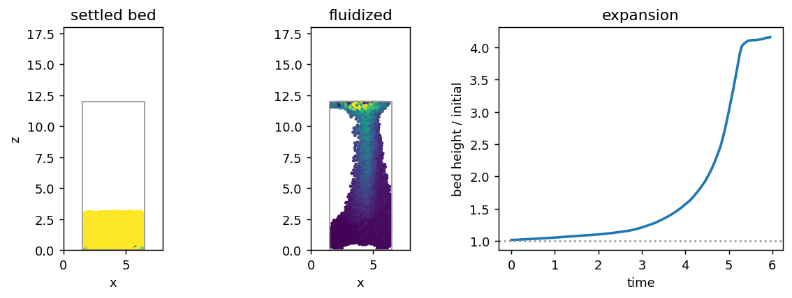
Sweeping the gas velocity traces the classic fluidization curve: flat while the bed is fixed, then rising once U clears U_mf.
def final_height(U, steps=80):
    s = make_flow(U); d = make_dem(pos0)
    c = CfdDem(s, d, fluid_dt=0.05, mu=mu_g, rho=rho_g, radius=rp, drag="gidaspow",
               dem_substeps=20, periodic=(False, False, False), move_particles=True, porous=True)
    for _ in range(steps): c.step()
    return bed_top(c)

Us = [0.0, 0.04, 0.08, 0.12, 0.16]
Hs = [final_height(U) for U in Us]
plt.figure(figsize=(4.6, 3.2))
plt.plot(Us, Hs, "o-", lw=2); plt.axhline(Hs[0], ls=":", c="0.6", label="fixed-bed height")
plt.xlabel("superficial gas velocity U"); plt.ylabel("bed height (95th pct)")
plt.title("fluidization curve"); plt.legend(); plt.tight_layout()
print("bed height vs U:", {U: round(h, 2) for U, h in zip(Us, Hs)})
bed height vs U: {0.0: 2.89, 0.04: 3.08, 0.08: 3.56, 0.12: 4.37, 0.16: 5.55}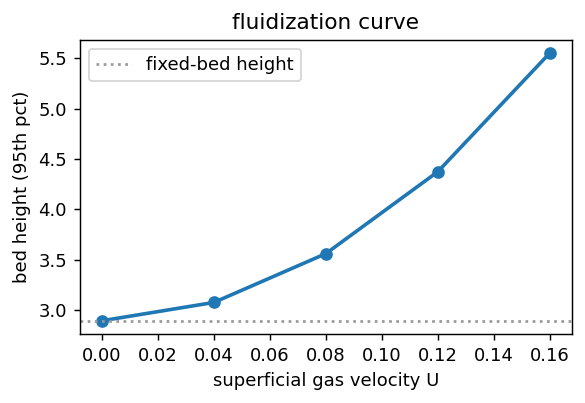
The real thing: reproducing an X-ray tomography benchmark with a million beads
For the engineering-scale run we reproduce a published, experimentally measured system: the cylindrical gas-fluidized bed of Verma et al. (2014), imaged at Helmholtz-Zentrum Dresden-Rossendorf with ultrafast electron-beam X-ray tomography (1000 cross-sections per second, two planes 11 mm apart) and simulated by the authors with a two-fluid model. Their glass case at bed aspect ratio 1.0 is, fortuitously, an almost exactly one-million-particle system — and every parameter is documented:
| Verma et al. (Tables 5–6) | here | |
|---|---|---|
| column | D = 0.1 m cylinder, 0.36 m simulated | cut-cell IBM cylinder, 32 cells across (h = 3.1 mm ≈ 3.1 dp), 0.36 m |
| particles | glass, dp = 1.0 mm, ρ = 2526 kg/m³ | 965,000 spheres → H₀ = 0.10 m (AR = 1.0) |
| collisions | en = 0.86 (their calibrated value) | e = 0.86, μ = 0.1 (glass–glass) |
| gas | air, uniform inflow through a porous plate | inflow floor at the superficial velocity, outflow roof |
| velocity | U = 1.5 Umf, Umf = 0.68 m/s | identical |
| drag | van der Hoef / Beetstra lattice-Boltzmann closure | drag="beetstra" |
| duration | 20 s, first 1 s discarded | 6.5 s, first 1 s discarded |
The canonical run lives in make_verma_bed.py (a ~20 h single-GPU job: settle, then 16,250 coupled steps of 0.4 ms with 20 DEM substeps each). It writes the porosity time series at the paper’s measurement planes plus full 3-D porosity frames; the cells below post-process them exactly the way the paper post-processes its tomograms — bubbles are connected ε > 0.7 regions in a horizontal plane (with linear sub-grid interpolation), the equivalent diameter is the number average of \(\sqrt{4A/\pi}\), and the rise velocity comes from cross-correlating the two planes of a pair.
from scipy import ndimage
fb = np.load("verma_bed.npz")
planes, kzv, h_m = fb["planes"], fb["kz"], float(fb["h_m"])
dt_frame = float(fb["dt"]) * int(fb["sample_every"])
inmask = fb["inmask"]
Pn = planes[int(round(1.0 / dt_frame)):]              # discard t < 1 s, like the paper
mz = ndimage.zoom(inmask.astype(float), 4, order=1) > 0.5
cell_area, min_area = (h_m / 4) ** 2, 2 * h_m ** 2

def bubbles(plane):
    z = ndimage.zoom(plane, 4, order=1)               # their linear boundary interpolation
    lab, n = ndimage.label((z > 0.7) & mz)
    if n == 0: return []
    A = ndimage.sum_labels(np.ones_like(z), lab, np.arange(1, n + 1)) * cell_area
    return list(np.sqrt(4 * A[A >= min_area] / np.pi))

De_planes, vb = {}, {}
for jlo, jhi, H in [(0, 1, 0.05), (2, 3, 0.10)]:
    allD = [d for fr in Pn for d in bubbles(fr[jlo])]
    De_planes[H] = (np.mean(allD), np.std(allD), len(allD))
    a = Pn[:, jlo][:, inmask]; b = Pn[:, jhi][:, inmask]
    a = a - a.mean(axis=0); b = b - b.mean(axis=0)    # their Eq 7, area-weighted CCF
    R = np.array([np.mean(np.sum(a[:len(a)-n] * b[n:], axis=1)) for n in range(40)])
    n0 = int(np.argmax(R[1:]) + 1)
    num, den = R[n0-1] - R[n0+1], 2 * (R[n0-1] - 2*R[n0] + R[n0+1])
    n0 = n0 + max(-0.5, min(0.5, num/den if den else 0.0))
    vb[H] = (kzv[jhi] - kzv[jlo]) * h_m / (n0 * dt_frame)
for H in (0.05, 0.10):
    De, sd, n = De_planes[H]
    print(f"H = {H*100:.0f} cm:  De = {De*1e3:4.1f} mm (±{sd*1e3:.0f}, n={n})   "
          f"bubble rise = {vb[H]:.2f} m/s")
H = 5 cm: De = 35.2 mm (±22, n=2355) bubble rise = 0.63 m/s
H = 10 cm: De = 41.5 mm (±26, n=3778) bubble rise = 0.89 m/sThe bubble-size profile — the paper’s central figure — comes from the stored 3-D frames (precomputed by compute_verma_profile.py), with their X-ray measurements and TFM digitized from their Figure 14 and the two literature correlations they compare against:
prof = np.load("verma_profile.npz")
Hp, Dep = prof["H"], prof["De"]
sel = Hp <= 0.115                                     # our AR = 1.0 bed surface; above is freeboard
Hexp = np.array([0.040, 0.050, 0.095, 0.100, 0.190, 0.200])
Dexp = np.array([0.022, 0.026, 0.032, 0.038, 0.039, 0.040])
Htfm = np.array([0.02, 0.04, 0.06, 0.08, 0.10, 0.12, 0.14, 0.16, 0.18, 0.20])
Dtfm = np.array([0.015, 0.019, 0.024, 0.028, 0.033, 0.036, 0.040, 0.043, 0.044, 0.045])
Hc = np.linspace(0.01, 0.20, 60); Uex = 0.5 * 0.68
Darton  = 0.54 * Uex**0.4 * Hc**0.8 * 9.81**-0.2
Werther = 0.00853 * (1 + 27*Uex)**(1/3) * (1 + 6.4*Hc)**1.21

fig, ax = plt.subplots(figsize=(6.4, 4.2))
ax.plot(Hp[sel], Dep[sel]*1e3, color="#2a6fdb", lw=2, label="peclet CFD-DEM (1M particles)")
for H in (0.05, 0.10):
    ax.plot(H, De_planes[H][0]*1e3, "o", color="#2a6fdb", ms=8)
ax.plot(Hexp, Dexp*1e3, "s", color="k", ms=6, label="X-ray experiment (Verma et al.)")
ax.plot(Htfm, Dtfm*1e3, "^-", color="0.55", ms=4, lw=1, label="their TFM")
ax.plot(Hc, Darton*1e3, "--", color="crimson", lw=1, label="Darton et al.")
ax.plot(Hc, Werther*1e3, "-", color="crimson", lw=1, label="Werther")
ax.set(xlabel="height above distributor H [m]", ylabel="equivalent bubble diameter $D_e$ [mm]",
       xlim=(0, 0.21), ylim=(0, 60))
ax.legend(fontsize=8); plt.show()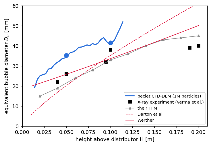
bins = np.arange(0.30, 1.02, 0.04)
fig, axs = plt.subplots(1, 2, figsize=(9, 3.4))
for j, H, c in [(0, 0.05, "#2a6fdb"), (2, 0.10, "#e08a1e")]:
    hist, _ = np.histogram(Pn[:, j][:, inmask].ravel(), bins=bins, density=True)
    axs[0].plot(bins[:-1] + 0.02, hist, "-o", ms=3, color=c, label=f"H = {H*100:.0f} cm")
axs[0].set(xlabel="porosity ε", ylabel="PDF"); axs[0].legend()
dPs, W_A = fb["dPs"], float(fb["W_over_A"])
td = np.arange(len(dPs)) * dt_frame
axs[1].plot(td, dPs, lw=0.8)
axs[1].axhline(W_A, color="crimson", ls="--", label="bed weight / area")
i0d = int(round(1.0 / dt_frame))
axs[1].set(xlabel="time [s]", ylabel="ΔP [Pa]"); axs[1].legend()
plt.tight_layout(); plt.show()
print(f"<dP>/(W/A) over t = 1–6.5 s: {dPs[i0d:].mean()/W_A:.2f}")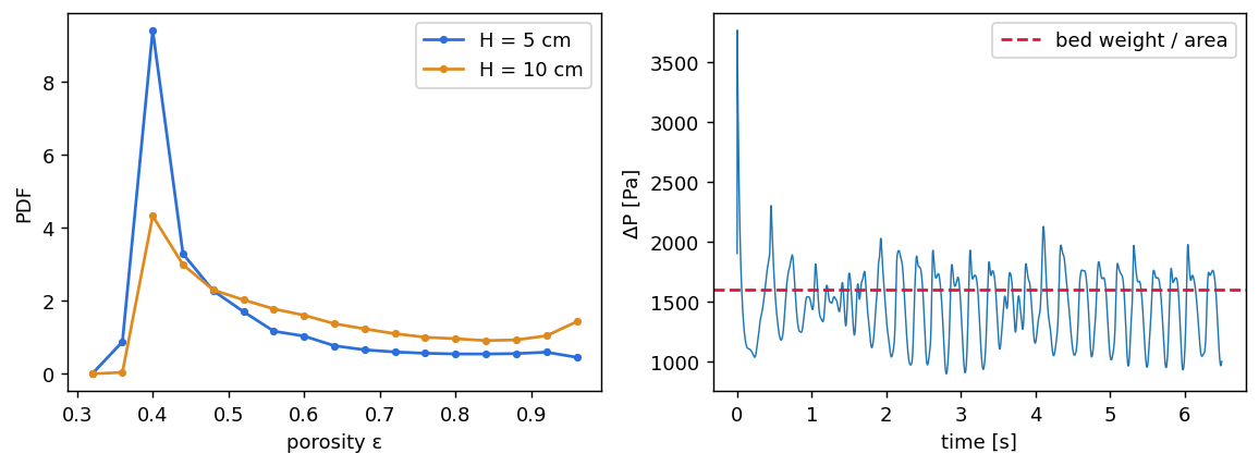
<dP>/(W/A) over t = 1–6.5 s: 0.92And the bubbles themselves, rendered as the ε = 0.7 isosurface — the same contour the paper draws in its Figure 6: small bubbles emerge near the distributor, coalesce into large central bubbles, and erupt through the domed, breathing bed surface.
How close is the reproduction? With no tuned parameters — geometry, material, restitution, velocity, and drag closure all taken from their tables, plus this suite’s documented defaults — the comparison stands as:
| quantity | CFD-DEM (here) | X-ray | their TFM |
|---|---|---|---|
| De at H = 10 cm | 41.5 mm | ≈ 38 mm | ≈ 33 mm |
| De at H = 5 cm | 35 mm | ≈ 26 mm | ≈ 20 mm |
| bubble rise at 5 cm | 0.63 m/s | ≈ 0.55 m/s | ≈ 0.45 m/s |
| bubble rise at 10 cm | 0.89 m/s | ≈ 0.60 m/s | ≈ 0.62 m/s |
| ⟨ΔP⟩ / (W/A) | 0.92 | — | — |
Higher in the bed the bubble size lands within ~10% of the measurement — from the large side, where the TFM approaches from the small side. Near the distributor we over-predict: the vigorous coalescence region produces many mid-size detections that the X-ray processing partially merges into its larger bubbles. The 10-cm rise velocity is high — 1 mm glass sits on the Geldart B/D border, where gas through-flow in large bubbles (which a discrete drag model resolves per particle) raises the apparent void propagation speed. The porosity PDFs agree on the bubble phase; the emulsion peak sits at our physically packed ε ≈ 0.40 versus ≈ 0.56 from their attenuation calibration. For a first-shot, no-tuning reproduction across five measured quantities, this is the kind of agreement that makes the benchmark worth keeping in the suite.
Performance
The full benchmark run — 965,000 grains, 119k fluid cells, 16,250 coupled steps of 0.4 ms with 20 XPBD substeps each — took 20.8 h on one RTX 5080, i.e. ~4.8 s per coupled step with a contact-rich packed bed and the cut-cell projection at every step. The coupling is device-resident end to end (void-fraction deposit, drag, reaction, and the DEM force buffer are zero-copy device views); the recorded diagnostics (two plane pairs at 2 ms, full 3-D porosity at 10 ms) are the only host traffic.
Adapt this yourself
- Change the drag law.
drag="wen_yu","di_felice","schiller_naumann","stokes","gidaspow"(the demo above),"beetstra","tang"(the benchmarks). Each is a device-inline correlation incoupling/src/drag.hpp; the porous mode applies the Model-Bβ/εconversion to any of them. - Change the vessel. The wall SDFs are ordinary functions — swap the cylinder for a cone (spouted bed), add a draft tube, or make the distributor a perforated plate.
- Go multi-rank. Build the
peclet-*-mpimodules, passflow.init_mpi/dem.init_mpithe same decomposition, andCfdDemruns the distributed deposit-fold + gather + DEM step. - Taller, wider, denser. The step cost is dominated by the DEM at ~0.5 s per million grains; the fluid grid is far from its limit.
Reproduce this
# CPU (OpenMP) — flow + dem + the coupling module, built from source against a Kokkos prefix:
tools/bootstrap_deps.sh host-openmp                      # one-time Kokkos/ArborX prefix
for m in flow dem coupling; do
  cmake -S $m -B $m/build -DCMAKE_PREFIX_PATH="$PWD/extern/install/host-openmp"; cmake --build $m/build -j
done
PECLET_LOCAL_BUILD="$PWD/flow/build:$PWD/dem/build:$PWD/coupling/build" \
  quarto render examples/fluidized-bed/index.qmd
# GPU (needed for the million-grain section): point CMAKE_PREFIX_PATH at
# extern/install/nvidia-cuda instead (nvcc on PATH) and pip install cupy-cuda13x pyvista imageio-ffmpeg.