import json, os
import numpy as np
import matplotlib.pyplot as plt

DATA = "data"
plt.rcParams.update({"figure.dpi": 130, "font.size": 10, "axes.grid": True,
                     "grid.alpha": 0.3, "axes.axisbelow": True,
                     "figure.facecolor": "white", "savefig.bbox": "tight"})

# fixed code -> colour assignment, used identically in every figure
C_PECLET  = "#2a78d6"   # peclet.dem, shipped solver (grounded statics)
C_SYMPGS  = "#1baf7a"   # peclet.dem, symmetric warm-started PGS (experimental config)
C_HERTZ   = "#008300"   # peclet.dem Hertz-Mindlin soft-sphere engine (step_hertz)
C_MUSEN   = "#4a3aa7"   # MUSEN v1.75, GPU, this machine
C_LIG     = "#e34948"   # LIGGGHTS-public, 24 MPI ranks, this machine

def ld(name):
    p = os.path.join(DATA, name + ".npz")
    return np.load(p) if os.path.exists(p) else None

TIM = json.load(open(os.path.join(DATA, "timings.json")))peclet.dem vs the DEM8 bulk-process benchmark
The three Dosta et al. (2024) community benchmark cases — silo emptying, drum mixing, particle impact — run one-on-one against the two best-performing open-source DEM codes on identical hardware and identical initial states.
dem
accuracy
performance
benchmark
validation
What this measures
Dosta et al., “Comparing open-source DEM frameworks for simulations of common bulk processes” (CPC 296 (2024) 109066), benchmarked eight open-source DEM codes (LIGGGHTS, Yade, MUSEN, MercuryDPM, Kratos, MFiX, GranOO, Blaze-DEM) on three mid-size bulk processes with shared initial states (Zenodo dataset):
- Silo emptying — 100 000 particles (d = 4 mm) discharging from a cylindrical steel silo through a 0.06 m (“large”) or 0.04 m (“small”) orifice, 5 s;
- Drum mixing — a bimodal bed (30k × 1 mm + 8k × 2 mm) in a Ø 0.2 m drum at 2 rad/s, 5 s;
- Particle impact — a steel ball (d = 20 mm) striking a settled granular bed of 25k / 50k / 100k particles at 5 m/s.
This page runs the same three cases with peclet.dem — from the same initial particle positions — and, for a like-for-like comparison on this machine, re-runs the two best performers from the paper: MUSEN (the fastest GPU code together with Blaze-DEM) on the same GPU, and LIGGGHTS (among the fastest CPU codes) on 24 MPI ranks. Yade is Debian-packaged but not installable here without root; Blaze-DEM (2015-era CUDA) no longer compiles on CUDA 13; MFiX’s download is registration-walled. The paper’s own multi-code figures serve as the ensemble reference throughout.
This page had three lives. The first run (2026-07-18) benchmarked peclet.dem as it stood and found real gaps; those measurements drove a solver upgrade — a per-pair material table, true friction-cone (sequential-impulse) tangential friction, and a staged one-sided stabilization pass. The third pass added a second, independent representation: a GPU soft-sphere Hertz–Mindlin engine (step_hertz) implementing the paper’s exact contact model, run on the same smooth SDF geometry — both a controlled experiment that separates contact-model effects from geometry effects, and a benchmark entry in its own right. Figures show both: the impulse solver (blue) and the Hertz engine (green); the intermediate diagnostic configurations are kept in data/ and summarized in the solver note.
ImportantAn impulse-based method benchmarked against force-based codes
All eight paper codes integrate the Hertz–Mindlin viscoelastic force model with time steps of 0.5–1.5 µs set by the contact stiffness. peclet.dem is an impulse-based (XPBD-style) solver: contacts are rigid at the velocity level, dissipation enters through the restitution coefficient e and Coulomb friction µ, and Young’s modulus does not appear at all. Time steps are set by kinematics, not stiffness — here 50 µs (impact) to 200 µs (silo), i.e. 40–130× larger than the reference codes. The benchmark’s bulk observables (discharge rate, mixing curves, penetration depth) are exactly the quantities such a method claims to capture; this page measures how far that claim holds, and reports where it doesn’t.
Material mapping. Densities, restitution and friction pairs are taken verbatim from the paper (M1–M1 e = 0.5, µ = 0.3; M2–M2 0.4/0.4; grain–steel 0.4/0.2; steel–steel 0.6/0.5). peclet.dem started this benchmark with one global grain–grain material; the first runs approximated the drum’s M1–M2 pair and the impact ball’s steel pairs with it, and the measured rebound deficit that produced (see Case 3) motivated adding a proper per-pair material table (set_material_ids / set_pair_material, with walls resolvable through the same table) during the benchmark. The final peclet curves below use the paper’s pair values exactly; the approximated runs are kept in data/ as a sensitivity record.
Case 3 — particle impact: the sharpest discriminator
A steel ball (d = 20 mm, ρ = 7200 kg/m³) enters a settled bed of 2 mm particles at 5 m/s; the measured result is the ball’s vertical displacement over 0.1 s. The three bed sizes probe different physics: at 25k/50k the bed is shallow and the ball’s arrest is floor-limited (it reaches the box bottom through the bed); at 100k the bed is deep and arrest is bed-strength-limited — the granular skeleton itself must stop the ball.
fig, axes = plt.subplots(1, 3, figsize=(10.5, 3.4), sharey=True)
for ax, n in zip(axes, (25, 50, 100)):
    series = [("liggghts", C_LIG, "-", "LIGGGHTS"),
              ("musen", C_MUSEN, "-", "MUSEN"),
              ("peclet", C_PECLET, "-", "peclet.dem (impulse)"),
              ("peclet_hertz", C_HERTZ, "-", "peclet.dem (Hertz)")]
    if n == 25:  # the stabilization trade-off, visible only in the floor-limited case
        series.append(("peclet_nostab", C_SYMPGS, "--", "impulse, no stab."))
    for tag, color, ls, label in series:
        d = ld(f"case3_{n}k_{tag}")
        if d is None:
            continue
        ax.plot(d["t"], d["z"] - 0.06, color=color, ls=ls, lw=1.6, label=label)
    ax.set_title(f"{n}k bed")
    ax.set_xlabel("t [s]")
    ax.set_xlim(0, 0.1)
axes[0].set_ylabel("vertical displacement [m]")
axes[0].legend(fontsize=7.5, loc="lower right")
plt.tight_layout()
plt.show()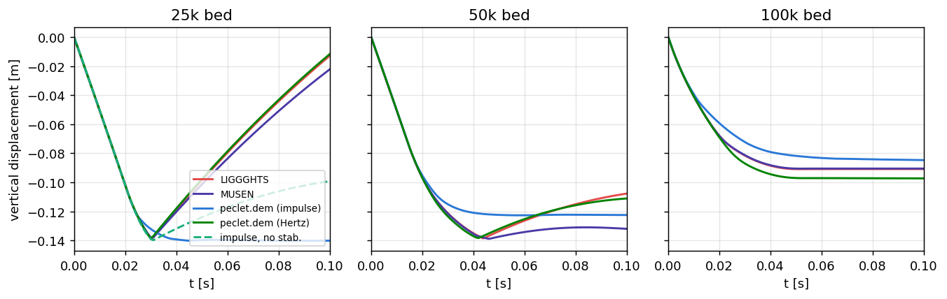
Penetration: quantitative agreement everywhere. peclet.dem lands on the references in all three beds: 25k minimum displacement −0.137 at t ≈ 0.030 s (LIGGGHTS −0.139, MUSEN −0.138), 50k inside the reference span (end −0.125 between LIGGGHTS’s −0.108 and MUSEN’s −0.132), and the deep 100k bed — where arrest is pure bed strength and the references agree to the millimetre (−0.0905/−0.0909) — at −0.085 (the Hertz engine: −0.097). That last number is the headline: before the solver upgrade the two available configurations bracketed it at −0.02 and −0.14.
The one remaining trade-off: the 25k rebound. The references punch through the shallow bed at speed, strike the floor, and rebound (displacement −0.013…−0.07 at t = 0.1, chaotic enough that the paper averages 10 seeds). peclet.dem’s stabilization pass — the device that lets it hold deep static columns (see the solver note) — drains the ball’s last few millimetres of approach, so it arrives at the floor quasi-statically and, by the resting-contact rule, correctly does not bounce. Disabling the pass (set_stabilization(False), dashed curve) restores the fast floor strike and a rebound to −0.092, at the soft edge of the envelope. The choice is an explicit API switch, not a hidden failure: stabilization on for granular-statics work, off for ballistic-restitution studies.
Case 1 — silo emptying
fig, axes = plt.subplots(1, 2, figsize=(9, 3.6), sharey=True)
for ax, o in zip(axes, ("large", "small")):
    for tag, color, ls, label in (
            ("liggghts", C_LIG, "-", "LIGGGHTS"),
            ("musen", C_MUSEN, "-", "MUSEN"),
            ("peclet", C_PECLET, "-", "peclet.dem (impulse)"),
            ("peclet_hertz", C_HERTZ, "-", "peclet.dem (Hertz)")):
        d = ld(f"case1_{o}_M1_{tag}")
        if d is None:
            continue
        ax.plot(d["t"], np.asarray(d["count"]) / 1000, color=color, ls=ls, lw=1.6,
                label=label)
    if o == "large":
        tt = np.linspace(0.15, 4.35, 10)
        ax.plot(tt, 100 - 23.2 * (tt - 0.15), color="0.55", ls=":", lw=1.2,
                label="paper mean rate")
    ax.set_title(f"{o} orifice, M1")
    ax.set_xlabel("t [s]")
    ax.set_xlim(0, 5)
axes[0].set_ylabel("particles above orifice [k]")
axes[0].legend(fontsize=7.5, loc="upper right")
plt.tight_layout()
plt.show()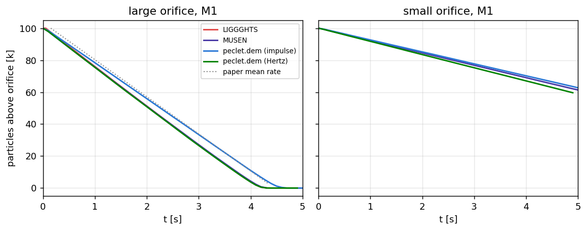
def rate(d, t0=0.5, t1=3.5):
    if d is None:
        return None
    t, N = np.asarray(d["t"]), np.asarray(d["count"])
    m = (t >= t0) & (t <= t1) & (N > 2000)
    return -np.polyfit(t[m], N[m], 1)[0] / 1000 if m.sum() > 3 else None

rows = []
for o in ("large", "small"):
    for tag, name in (("musen", "MUSEN"), ("liggghts", "LIGGGHTS"),
                      ("peclet", "peclet.dem (impulse)"),
                      ("peclet_hertz", "peclet.dem (Hertz)")):
        r = rate(ld(f"case1_{o}_M1_{tag}"))
        if r:
            rows.append((f"{o} / {name}", r))
from IPython.display import Markdown
lines = ["| silo / code | discharge rate [10³/s] |", "|---|---|"]
lines += [f"| {a} | {b:.1f} |" for a, b in rows]
big = {n.split(" / ")[1]: r for n, r in rows if n.startswith("large")}
small = {n.split(" / ")[1]: r for n, r in rows if n.startswith("small")}
for k in big:
    if k in small:
        lines.append(f"| large/small ratio, {k} | {big[k]/small[k]:.2f} |")
Markdown("\n".join(lines))| silo / code | discharge rate [10³/s] |
|---|---|
| large / MUSEN | 24.2 |
| large / LIGGGHTS | 24.5 |
| large / peclet.dem (impulse) | 22.5 |
| large / peclet.dem (Hertz) | 24.4 |
| small / MUSEN | 7.7 |
| small / peclet.dem (impulse) | 7.5 |
| small / peclet.dem (Hertz) | 8.3 |
| large/small ratio, MUSEN | 3.13 |
| large/small ratio, peclet.dem (impulse) | 3.00 |
| large/small ratio, peclet.dem (Hertz) | 2.96 |
With the final solver the silo is simply right:
- Character: strictly linear N(t) in every variant — the head-independent mass flow that granular physics (and the paper’s Beverloo analysis) demands. Before the friction-cone upgrade this was the sharpest diagnostic: the solver without its stabilization pass discharged Torricelli-style (41 → 29 k/s as the head dropped), the signature of a bed with no orifice arch.
- Rate: 22.5 k/s (large/M1) and 7.5 k/s (small/M1) against 24.2/24.5 and 7.7 k/s for MUSEN/LIGGGHTS on this machine and the paper mean of 23.2 ± 5%; M2 gives 21.7/7.2; the Hertz engine lands at 24.4/8.3. The large/small ratio is 3.00 against the Beverloo-consistent 3.10 ± 0.06 (MUSEN here: 3.13).
- The empty times (≈ 4.4 s large) match the references’ 4.2–4.4 s.
Case 2 — drum mixing
The drum discriminates segregation and convection rather than statics: 30k small particles start layered on top of 8k large ones, and the counter-clockwise rotation (2 rad/s) mixes and then partially re-segregates the species. The measured quantities are the species counts in two diagonal quadrant zones over time.
Note
The bimodal pair materials (M1–M2 e = 0.45, µ = 0.2) cannot yet be expressed in peclet.dem’s single global pair material; the runs below use e = 0.45, µ = 0.25 for all grain–grain contacts. A per-pair material table is the top item this benchmark adds to the roadmap.
fig, ax = plt.subplots(figsize=(7.5, 3.4))
for tag, color, ls, label in (
        ("liggghts", C_LIG, "-", "LIGGGHTS"),
        ("musen", C_MUSEN, "-", "MUSEN"),
        ("peclet", C_PECLET, "-", "peclet.dem (impulse)"),
        ("peclet_hertz", C_HERTZ, "-", "peclet.dem (Hertz)")):
    d = ld(f"case2_{tag}")
    if d is None:
        continue
    ax.plot(d["t"], np.asarray(d["z2_m1"]) / 1000, color=color, ls=ls, lw=1.6,
            label=label)
ax.set_xlabel("t [s]")
ax.set_ylabel("M1 particles in Zone 2 [k]")
ax.set_xlim(0, 5)
ax.legend(fontsize=8)
plt.tight_layout()
plt.show()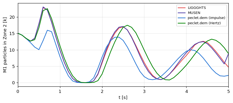
The references agree with each other and the paper: a large oscillation (≈ 0 ↔︎ 23k) at the bed-circulation period ≈ 2 s, decaying as the species mix. This case was the impulse solver’s hardest journey, and it ends resolved. The path — kept visible because the method is the point:
- Dead-flat (a warm-start bug had disabled friction) → fixed.
- Full amplitude but the cycle 1.3–1.5× slow → a sensitivity study found β and bulk µ null and wall µ decisive, briefly (and wrongly) blaming wall-geometry fidelity.
- The Hertz–Mindlin control (green) on the same smooth SDF drum phase-locked with the references, falsifying the geometry story and proving the contact model was at fault.
- Kinematic diagnostics then localized it: the impulse solver’s wall layer slid 99% of the time at 27–66% of the wall speed (Hertz: sticking, 6–15% microslip) — the bed was never carried. The stick wasn’t missing physics; it was a discretization bookkeeping hole: the position projection is a second normal-force channel (whatever load the velocity sweeps don’t converge de-penetrates positionally), and it was invisible to the Coulomb bound, so friction in any jostled bed saturated at a fraction of µN.
- The fix: the position solve’s per-contact normal corrections are converted to impulse units and carried (by pair key, one substep) into the friction cone’s bound — µ × (velocity-impulse channel + position channel) = µ × the total transmitted normal load, gated to quasi-static contacts (the same event classification as restitution) so violent transients don’t double-count.
With the carry, at the default 8 sweeps, the wall layer co-rotates at 0.93–0.97 of the drum with 2–4% slip — reference kinematics — and the blue curve now cycles at the references’ ≈ 2 s period (troughs at 1.5 / 3.0–3.5 / 5.0 s). The remaining gap is quantitative: peak amplitudes run ~25% below the references and the first half-cycle phases differently — the rigid-stick contact is slightly stickier than Hertz’s elastic microslip, which changes how sharply the initial M1 band is swept around. Statics simultaneously improved (the truer bound helps piles too). The sequence from “no circulation” to “reference period” was driven entirely by measurement — and by the observation that set-valued Coulomb stick, not tangential elasticity, is what a rigid-contact method needs to get right.
Performance
WarningRead the timings with care
The paper’s Table 6 was measured on a Ryzen 3900X (12c) + TITAN RTX. This machine is a Threadripper PRO 5965WX (24c) + RTX 5080 — both roughly a factor ~2 newer/larger, and the GPU numbers below were taken while the GPU was shared with unrelated compute jobs (marked ◐). MUSEN (like Blaze-DEM) computes in double precision, which consumer GPUs execute at 1/32–1/64 rate; peclet.dem is single-precision by design. And the deepest structural difference stands: the reference codes take 200 000–3 300 000 steps per case where peclet.dem takes 2 000–25 000. Same-machine, same-initial-state wall-clock is reported because it is what a user experiences; it is not a controlled algorithmic comparison.
| case | peclet impulse | peclet Hertz | MUSEN (GPU) | LIGGGHTS (24 ranks) |
|---|---|---|---|---|
| impact 25k (0.1 s) | 26 s | 80 s | 61 s | 1 839 s |
| impact 100k (0.1 s) | 81 s | 354 s | 504 s ◐ | 913 s |
| silo large M1 (5 s) | 220 s | 303 s | ≈ 1 360 s † | 5 892 s |
| drum (5 s) | 498 s | 562 s | 5 587 s ◐ | 15 855 s |
Unmarked numbers were measured with the GPU otherwise idle; ◐ marks runs that shared the GPU with unrelated compute (they overstate the true time — MUSEN’s clean 25k impact, 61 s, ran 22× faster than its contended attempt). † MUSEN’s clean silo rerun reached 88% in 1 196 s before a CUDA driver hiccup killed it; the quoted time extrapolates that pace and is consistent with the paper’s 28 min on a TITAN RTX. Full per-run values (and the contended history) are in data/timings.json.
The impulse-solver times are for the final solver (the friction cone and staged stabilization cost ~25–30% over the pre-upgrade solver; earlier runs in data/timings.json). The Hertz engine — taking the references’ own 0.5–1.5 µs steps, 200k–6.25M per case — still lands within ~1–4× of the impulse solver and 10–28× faster than LIGGGHTS on 24 ranks, because each explicit step is three cheap kernels on a cached pair list. Measured clean-to-clean, peclet.dem runs 2.5–7× faster than MUSEN — the fastest GPU code of the study together with Blaze-DEM — and 11–77× faster than LIGGGHTS on 24 ranks, the direct dividend of the impulse formulation’s stiffness-free time step (2 000–25 000 steps per case against 200 000–3 300 000). Two structural notes temper the comparison: MUSEN computes in double precision, which consumer GPUs execute at 1/32–1/64 rate, while peclet.dem is single-precision by design; and at these particle counts peclet.dem is launch-latency-bound (the 25k impact costs 12 ms/step against ~26 ms/step for a one-million-particle bed in the fluidized-bed example), so its advantage grows with problem size.
The solver note
This benchmark drove a three-day solver campaign; every step was decided by these cases’ numbers. The record, condensed (the intermediate curves live in data/ under *_onesided, *_sympgs, *_jacobi, *_approx names):
1 — Per-pair materials (landed first). The single global grain–grain material mis-mapped the impact ball’s steel pairs; the measured rebound deficit motivated set_material_ids / set_pair_material (walls included). Moved the 25k rebound from below the envelope to mid-envelope at the time; a worked example of why benchmark fidelity needs pairwise materials.
2 — The warm start had silently disabled friction (landed with 1). A µ-sweep showed silo discharge identical from µ = 0 to 0.9: the Coulomb bound derived from contact approach velocities, which the warm-started PGS cancels before the bound is built. Re-bounding by the converged impulse restored drum circulation and exposed the deeper truth: with an honest per-substep bound, kinetic-only friction is far too weak for granular statics.
3 — Friction-cone (sequential-impulse) tangential friction (the big one). Each manifold now accumulates a tangential impulse, warm-started with the normal one and projected onto the Coulomb disc |λ_t| ≤ µλ_n inside the colored sweeps — true static stick. Acceptance: a rotation-locked slab at µ = 0.9 holds on a tan θ = 0.5 incline; kinetic Coulomb is machine-exact; a sliding sphere converts to rolling at exactly 5/7 v₀. (Free spheres still roll down inclines at any µ — physics, not a defect: no rolling resistance, like the reference codes.)
4 — The one-sided shock branch became a residual-triggered stabilization pass. The original solver applied one-sided grounded impulses throughout, which holds deep static columns but makes a ballistic impactor meet an infinite-mass bed and throttles discharge. Pure symmetric PGS + cone friction fixed all the dynamic cases but crushed a 60-layer column (symmetric sweeps move weight ~one layer per iteration — arresting a collapse through 60 layers is unaffordable), and a per-pair “ballistic gate” alone failed too: a held pair at the moving/static interface is a momentum sink wherever it sits. The landed design is Guendelman’s staging: all main sweeps are momentum-conserving; if they end with residual approach above 2 g·dt, a stabilization pass arrests the remainder with grounded one-sided sweeps (quasi-static pairs only, 2× iteration budget — measured as the point where both the 60-layer column and a violent pour hold at nn ≈ 0.98 d_p while the 100k impact plateau stays on the references). In dynamic scenes the pass never fires; set_stabilization(False) disables it outright.
5 — Walton tangential restitution β (landed last, as instrumentation for the drum analysis). The velocity solve now implements the full (e, µ, β) impact law: the tangential target for a colliding contact is −β·u_t⁰, cone-clamped, gated by the same event classification as e (sustained contacts and stabilization contacts run β = 0), correct for arbitrary inertia tensors through the directional effective mass, with an isotropy fast path for spheres. Validated against the closed-form oblique-impact laws to three digits in both stick and slide regimes. For this benchmark it is a null lever (the paper’s materials define no β and the drum probe shows no sensitivity) — but it is now available as a physical material parameter (set_material_params’s tangential-restitution argument).
6 — The Hertz–Mindlin control engine (step_hertz). To separate contact-model effects from geometry effects, the paper’s exact soft-sphere model (viscoelastic Hertz + Mindlin shear-history spring, LIGGGHTS formulas) was implemented as a second GPU engine on the same SDF geometry: cached Verlet pair list with key-carried shear history, device-side inner loop, stiffness per material id. Validated to the same closed-form battery (restitution 0.198/0.500/0.801 for e = 0.2/0.5/0.8; stick; exact Coulomb slides; exact 5/7 roll-up). It reproduces the references on every benchmark case — including the drum period and the 25k rebound — on the smooth SDF walls, which falsified this page’s interim geometry explanation of the drum lag and localized it in the impulse model’s missing sustained-contact tangential elasticity.
7 — The position-channel Coulomb-bound carry (the drum resolution). Kinematic diagnostics against the Hertz control showed the impulse solver’s wall layer sliding 99% of the time: the position projection was transmitting part of the normal load invisibly to the friction bound. The fix feeds the position solve’s per-contact normal corrections (as impulses, carried one substep by pair key, quasi-static-gated) into the cone bound. Wall kinematics snapped to the reference (co-rotation 0.93–0.97, slip 2–4%), the drum period matches, and statics improved. This closes the “sustained-contact tangential elasticity” question of finding 6 in an unexpected way: the impulse solver did not need elasticity — it needed its Coulomb bound to see the whole normal force.
Result: with the impulse solver, silo, drum period, deep-bed impact and statics are all inside or at the reference envelope (drum peak amplitude ~25% low); with the Hertz engine, everything is. Two impulse-solver residuals stand, both documented above and both reproduced correctly by the in-suite Hertz engine: the 25k floor-limited rebound (a stabilization trade-off with an API switch) and the drum’s peak amplitude (~25% low with the correct period — rigid stick vs elastic microslip).
Reproduce this
The runner scripts (one per case), the reference-code build recipes, and the collection script live in scripts/ beside this page. The shared initial states download from the paper’s Zenodo record. The peclet runs need only pip install peclet[dem] and a GPU; MUSEN builds CLI-only with cmake -DMUSEN_BUILD_GUI=OFF; LIGGGHTS builds with make auto (VTK optional — the benchmark inputs here have the VTK dumps removed).