Multi-GPU scaling: turbulent channel DNS on Snellius H100
5.5 Gcell-updates/s on 32 H100s at 86 % weak efficiency, with the pressure solve pinned at 6.0 iterations from 1 GPU to 32 — and a measurement of what a wall-bounded DNS costs that a periodic benchmark cannot tell you.
This is the performance companion to the wall-bounded turbulence example, which is about reproducing the Moser–Kim–Mansour channel-flow statistics. The question here is what that DNS costs across many GPUs, and what sets the limit.
The instrument, the machine and the methodology are shared with the parallel-scaling study — same per-phase timers, same Snellius gpu_h100 partition, one MPI rank cgroup-bound to each GPU with GPU-aware MPI. What changes is the physics: walls instead of periodicity everywhere.
How you scale a channel
A periodic benchmark scales by tiling: add GPUs, add copies of the same vortex, every rank keeps solving an identical problem. A channel has walls in the wall-normal direction, so it can only grow in the two periodic directions — but that is legitimate, and worth being precise about why.
The DNS is streamwise-periodic with a body force, so there is no inflow, no outflow and no streamwise development: the flow is statistically homogeneous in x by construction. What the box length must satisfy is decorrelation — long enough that a structure does not interact with its own periodic image. Past a few correlation lengths the single-point statistics stop depending on the box, and extra length simply adds independent realisations. So replicating the box is the channel analogue of tiling vortices: rung N is the same turbulence, with more copies of it.
This ladder replicates one 1024 × 160 × 320 box (Lx = 12.8H, Lz = 4.0H, Δ⁺ = 2.25 — the MKM box at this resolution) alternately in the two periodic directions:
| GPUs | tiles | grid | Mcells | Mcells/GPU |
|---|---|---|---|---|
| 1 | 1×1 | 1024×160×320 | 52.4 | 52.4 |
| 2 | 2×1 | 2048×160×320 | 104.9 | 52.4 |
| 4 | 2×2 | 2048×160×640 | 209.7 | 52.4 |
| 8 | 4×2 | 4096×160×640 | 419.4 | 52.4 |
| 16 | 4×4 | 4096×160×1280 | 838.9 | 52.4 |
| 32 | 8×4 | 8192×160×1280 | 1677.7 | 52.4 |
Exactly 52.4 M cells per GPU at every rung, identical Δ⁺ and dt, unchanged CPG driving force, and every dimension rich in factors of two — which matters more than it sounds, see below. Load imbalance is 1.000 at every rung.
The curve
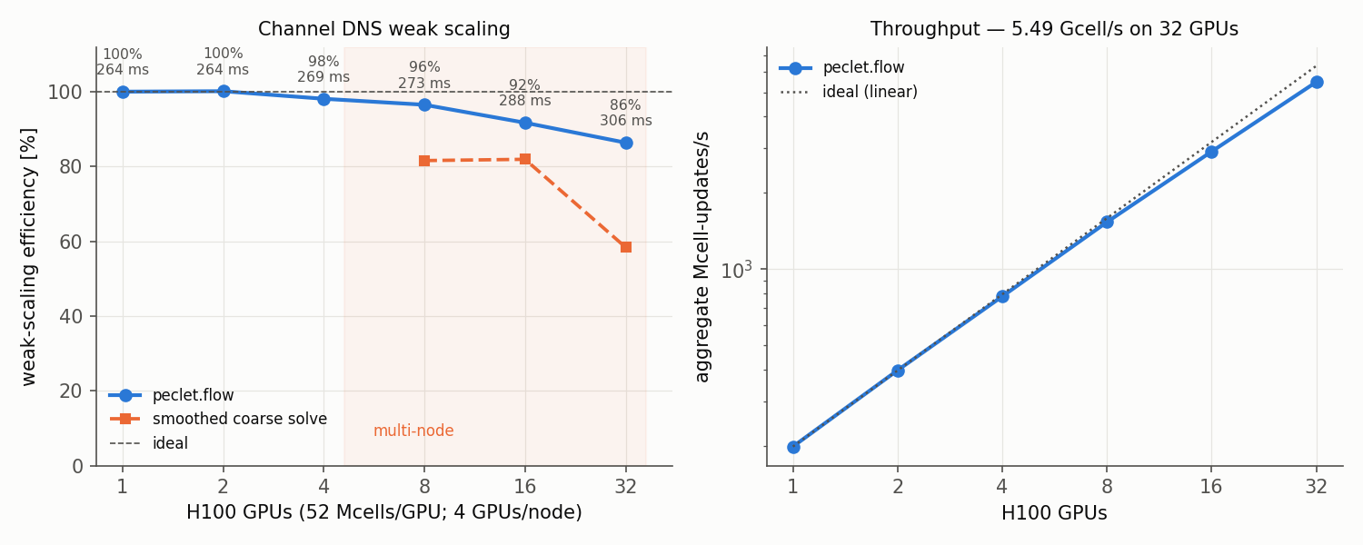
| GPUs | ms/step | pressure iters/step | Mcell/s | weak efficiency |
|---|---|---|---|---|
| 1 | 263.9 | 6.00 | 199 | 100 % |
| 2 | 263.6 | 6.00 | 398 | 100 % |
| 4 | 269.0 | 6.00 | 780 | 98 % |
| 8 | 273.5 | 6.00 | 1534 | 96 % |
| 16 | 287.8 | 6.00 | 2915 | 92 % |
| 32 | 305.6 | 6.00 | 5490 | 86 % |
5.5 Gcell-updates/s on 32 H100s at 86 % weak efficiency, with the pressure solve pinned at exactly 6.00 iterations per step from one GPU to thirty-two. A 1.68-billion-cell channel advances in 306 ms per step against 264 ms for a 52 M-cell one on a single GPU.
Where the step goes
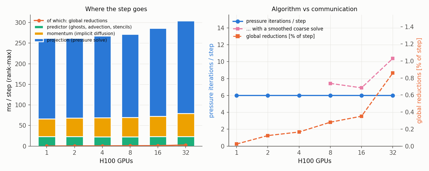
Communication is not the limit: the pressure solve’s global reductions run from 0.06 ms at 1 GPU to 2.6 ms at 32 — 0.02 % to 0.86 % of the step — and the reduction count is constant at 33 per step rather than growing. Load imbalance is 1.000 throughout.
The 14 % that is lost by 32 GPUs is entirely per-iteration cost, not more iterations:
| 1 GPU | 32 GPUs | |
|---|---|---|
| predictor | 23.1 ms | 23.4 ms |
| momentum | 43.0 ms | 55.7 ms |
| projection | 196.3 ms | 224.9 ms |
| — per pressure iteration | 32.7 ms | 37.5 ms |
| global reductions | 0.06 ms | 2.62 ms |
The predictor is flat. The projection does the same 6 iterations at every rung and each costs 15 % more, which is halo exchange inside the smoother and matvec. The momentum solve picks up one extra sweep at 32 GPUs (9 → 10) on top of a 17 % per-sweep increase. That is the healthy kind of weak-scaling loss — surface-to-volume, not algorithm.
What makes it work: the coarse-level solve
A V-cycle converges at a rate independent of the domain only if its coarsest level is effectively solved, and a distributed geometric hierarchy cannot always get there. An axis stops coarsening once it turns odd, and under MPI once any rank’s block turns odd — so the floor is roughly one cell per rank. At fixed cells/GPU the per-rank block is constant, so the coarsest global grid grows with the rank count no matter how many levels you request. Asking for more depth is a no-op past that point; the fix is to agglomerate the coarsest level onto a global operator and solve it there.
Running the identical ladder both ways isolates it:
| GPUs | agglomerated bottom | smoothed bottom | |
|---|---|---|---|
| 8 | 273.5 ms, 6.00 iters | 323.5 ms, 7.42 iters | 1.18× |
| 16 | 287.8 ms, 6.00 iters | 322.2 ms, 6.90 iters | 1.12× |
| 32 | 305.6 ms, 6.00 iters | 452.0 ms, 10.38 iters | 1.48× |
Without it the iteration count climbs with the rank count and weak efficiency falls to 58 % at 32 GPUs; with it, iterations do not move at all. The same effect is visible on a single GPU with no MPI in sight — lengthening a 2048 × 64 × 64 channel and varying only the depth:
| levels | smoothed bottom | agglomerated bottom |
|---|---|---|
| 4 | 13.5 iters, 167 ms | 4.0 iters, 112 ms |
| 6 | 6.0 iters, 91 ms | 4.0 iters, 69.5 ms |
| 12 (full geometric depth) | 4.4 iters, 77.2 ms | 4.4 iters, 77.1 ms |
An exact coarse solve is depth-independent, and a shallow hierarchy over it beats a deep one — the extra levels cost more than the coarse solve they replace. The criterion is the coarsest grid’s largest extent, not its cell count: a 64 × 2 × 2 bottom is only 256 cells and still costs 6.0 iterations against 4.0, because a point smoother needs O(L²) sweeps to damp a wavelength of L cells.
Select it with set_pressure_bottom("auto"), which agglomerates exactly when the coarsest grid exceeds four cells on any axis. The gathered operator is keyed by global cell id, so it is decomposition-independent by construction — measured, a 6-rank run agrees with a single-rank one to 4.5 × 10⁻¹⁶.
Grid dimensions are the single biggest lever
The multigrid coarsens each axis independently and only while that axis is even, so a dimension’s usable depth is its number of factors of two — and an odd dimension never coarsens at all. Measured on one GPU, 384 × 128 × N, everything else held:
| spanwise cells | halvings | pressure iters/step | ms/step |
|---|---|---|---|
| 256 | 8 | 5.0 | 120 |
| 250 | 1 | 9.8 | 195 |
| 255 | 0 | 16.2 | 329 |
One odd number costs 3.2×, with no MPI involved. A channel box derived the natural way — nx = round(2π·ny), nz = round(2π/3·ny) — lands on 1508 × 240 × 503, where the streamwise axis halves twice, the wall-normal four times, and the spanwise never. Round the grid to numbers rich in factors of two before anything else. flow ships a checker that needs neither a GPU nor a job:
python scripts/check_decomposition.py --grid 1508,240,503 --levels 5 --np 4 --walls --verboseRefining instead of replicating
Replicating answers “how efficiently does the machine run this solver”. The other question a DNS user asks is “can more GPUs buy me a finer DNS in the same wall-clock”, which is a different ladder: hold the box and refine it, so Δ⁺ goes 2.25 → 0.70 across 1–32 GPUs at ~46 M cells/GPU.
| GPUs | 1 | 2 | 4 | 8 | 16 | 32 |
|---|---|---|---|---|---|---|
| ms/step | 237 | 221 | 322 | 410 | 482 | 700 |
| pressure iters/step | 6.0 | 6.0 | 7.6 | 9.2 | 12.9 | 18.6 |
| weak efficiency | 100 % | 93 % | 75 % | 58 % | 43 % | 32 % |
That curve decays, and the decay is again the iteration count — but here, unlike the replicated ladder, the coarse solve is not what causes it. Re-running the identical ladder with the agglomerated bottom changes essentially nothing:
| GPUs | 1 | 2 | 4 | 8 | 16 |
|---|---|---|---|---|---|
| iters, smoothed bottom | 6.00 | 6.00 | 7.60 | 9.20 | 12.85 |
| iters, agglomerated bottom | 6.00 | 6.00 | 7.60 | 9.22 | 12.85 |
| ms/step, agglomerated | 237 | 218 | 318 | 417 | 462 |
It is not a no-op that failed to engage: the coarsest grid on these rungs runs 15 to 72 cells across, well past the threshold, and forcing agglomeration explicitly gives the same 12.85. The bottom simply is not the limit here.
Three things are therefore ruled out. Communication — 0.03 to 0.77 % of the step. The decomposition — one fixed grid on 1/2/4/8 GPUs holds iterations at 24.7 / 25.8 / 24.2 / 23.9, flat. The coarse level — the table above. What remains is the refinement itself, and that reproduces with no MPI in sight: on a single GPU, refining the same 6:1:2 box from Δ⁺ = 11.25 to 3.75 takes the solve from 4.0 to 5.0 iterations, the same trend the ladder continues to 12.85 at Δ⁺ = 0.94.
So refining this wall-bounded problem genuinely costs more iterations, and the GPU count is incidental. Two candidates remain unseparated: the V-cycle not being perfectly resolution-independent on a walled domain, and the flow itself changing as it becomes better resolved — a Δ⁺ = 2.25 field and a Δ⁺ = 0.70 field are not the same turbulence, and the pressure solve sees whatever divergence the velocity field hands it. Distinguishing them needs a fixed, converged flow field re-solved at several resolutions, which is not this measurement.
The honest summary is that the replicated ladder measures the machine and the refinement ladder measures the method, and only the first is a parallel-efficiency number.
Strong scaling: the same DNS, faster
Fixed 46.4 M-cell box, more GPUs:
| GPUs | 1 | 2 | 4 | 8 |
|---|---|---|---|---|
| ms/step | 830 | 486 | 301 | 227 |
| speed-up | 1.00× | 1.71× | 2.75× | 3.66× |
| efficiency | 100 % | 85 % | 69 % | 46 % |
| Mcells/GPU | 46.4 | 23.2 | 11.6 | 5.8 |
3.7× on 8 GPUs with the per-GPU problem down to 5.8 M cells; the falloff is the local work shrinking toward fixed per-step overheads, not the pressure solve — iterations are flat across this sweep.
Reproducing
The run pack is benchmarks/channel-scaling/snellius/ — one job per rung, resumable, mode and result tag as positional arguments:
sbatch --nodes=8 chan_weak_gpu.sh tile        # the replicated ladder (+ smoothed-bottom companions)
sbatch --nodes=4 chan_weak_gpu.sh refine      # the refinement ladder
sbatch --nodes=2 chan_weak_gpu.sh strong      # fixed-box strong scaling
Every run writes a JSON with the per-phase timers, iteration counts, reduction time and count and the full block map; all of them are in results/snellius-h100/, and plot_scaling.py regenerates the figures from them. The driver is the production DNS driver channel_dns_mpi.py — the benchmark runs the same code path as a real run, not a stripped-down kernel.