import importlib.util, os, subprocess, sys
_local = os.environ.get("PECLET_LOCAL_BUILD")
if _local:
    for p in _local.split(os.pathsep):
        sys.path.insert(0, p)
elif importlib.util.find_spec("peclet") is None:
subprocess.run([sys.executable, "-m", "pip", "install", "-q", "peclet"], check=True)Pore-network extraction: from DNS to throat conductances
Watershed the SDF into pores, then read exact throat flow rates and pore pressures straight off a resolved Stokes solution.
pnm
flow
porous-media
SDF
network
 Runs on a free Colab CPU runtime — the first cell installs
 peclet from PyPI.
What you’ll learn
Pore-network models (PNMs) replace a resolved porous-medium flow by a graph: pores (the wide places) connected by throats (the constrictions), each throat carrying a flow rate driven by the pressure difference between its pores. The hard part is getting that graph — and its flow data — consistently from a real geometry and a real flow field.
peclet.pnm does both on the voxel grid the DNS already lives on:
- Extraction — a marker-controlled watershed of the signed-distance field (SDF) segments the pore space into basins around each local maximum (
extract_pore_network). - Network flow — given a converged
peclet.flowsolution on the same grid, every throat’s flow rate is the sum of the solver’s own conserved face fluxes over the pore-pore interface, and every pore’s pressure is interpolated at its center (extract_network_flow).
Because the throat surfaces are made of the same staggered-MAC faces whose fluxes the pressure projection conserves, the bookkeeping is exact: summed around any pore, the throat flows cancel to the solver’s tolerance. That per-pore mass residual is returned with the network — a built-in correctness check you should always look at.
A periodic sphere packing
A jittered simple-cubic packing of overlapping solid spheres: the interstices form one pore per lattice cell, connected to its neighbours through the gaps between spheres. The SDF is positive in the pore space, negative in the solid (the suite convention), periodic in all directions.
import numpy as np
import matplotlib.pyplot as plt
from peclet import flow, pnm

plt.rcParams.update({"figure.dpi": 130, "font.size": 10, "axes.grid": True,
                     "grid.alpha": 0.3, "axes.axisbelow": True,
                     "figure.facecolor": "white", "savefig.bbox": "tight"})
BLUE, RED = "#1f77b4", "#d62728"
N, M = 64, 4 # grid cells, spheres per axis
pitch = N / M
R = 0.62 * pitch # overlapping -> real throats between the interstices
rng = np.random.default_rng(7)
x, y, z = np.meshgrid(*(np.arange(N, dtype=np.float64),) * 3, indexing="ij")
sdf = np.full((N, N, N), 1e30)
for ci in range(M):
for cj in range(M):
for ck in range(M):
c = pitch * (np.array([ci, cj, ck]) + 0.5) + rng.uniform(-0.12, 0.12, 3) * pitch
d = np.sqrt(sum(np.minimum(np.abs(w - cw), N - np.abs(w - cw)) ** 2
for w, cw in zip((x, y, z), c)))
sdf = np.minimum(sdf, d - R) # negative INSIDE the spheres (solid)
print(f"porosity {(sdf > 0).mean():.3f}")porosity 0.171Step 1 — extract the network
extract_pore_network runs the fused pipeline (pore detection → watershed segmentation → throat topology) in one call. Arrays follow the (Nz, Ny, Nx) C-order convention with z-y-x origin/spacing tuples.
sdf_zyx = np.ascontiguousarray(sdf.T, dtype=np.float32)
pores, seg_flat, conns = pnm.extract_pore_network(sdf_zyx, [0.0] * 3, [1.0] * 3)
seg = np.asarray(seg_flat, dtype=np.int32).reshape(N, N, N).T   # back to [x,y,z]
print(f"{len(pores)} pores, {len(conns)} label adjacencies")
93 pores, 320 label adjacenciesk = N // 2
fig, ax = plt.subplots(1, 2, figsize=(9, 4.2))
ax[0].imshow(sdf[:, :, k].T, origin="lower", cmap="RdBu", vmin=-6, vmax=6)
ax[0].set_title("SDF (slice z=N/2)")
m = np.ma.masked_less_equal(seg[:, :, k].T, 0)
ax[1].imshow(np.where(sdf[:, :, k].T > 0, 0, 1), origin="lower", cmap="Greys", vmin=0, vmax=3)
ax[1].imshow(m % 20, origin="lower", cmap="tab20", alpha=0.85)
for p in pores:
if abs(p.z - k) < 3:
ax[1].plot(p.x, p.y, "k.", ms=6)
ax[1].set_title("pore basins")
for a in ax:
a.set_xlabel("x"); a.set_ylabel("y"); a.grid(False)
plt.show()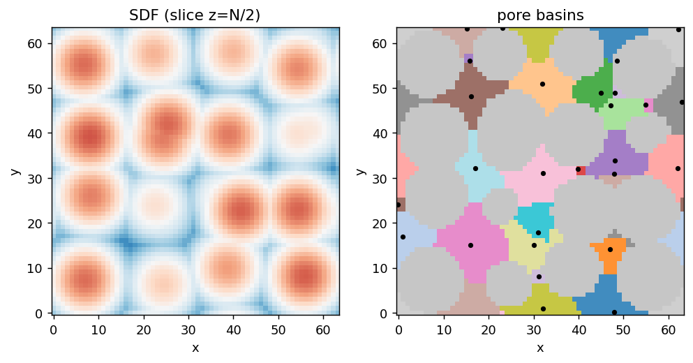
Step 2 — resolve the flow
A body force \(f_x\) drives creeping flow through the packing (the periodic equivalent of imposing a macroscopic pressure gradient \(\nabla p = -f_x\hat e_x\)). cutcell_pressure=True enables the cut-cell operator whose openness-weighted face fluxes are exactly what the network bookkeeping needs.
MU, FX = 0.05, 1e-3
s = flow.Solver(N, N, N)
s.set_rho(1.0); s.set_mu(MU); s.set_dt(100.0)
s.set_body_force(FX, 0.0, 0.0)
s.set_solid(np.asfortranarray(sdf), cutcell_pressure=True)
for _ in range(40):
    s.step()

u, v, w, p = s.get_uf(), s.get_vf(), s.get_wf(), s.get_p()
ox, oy, oz = s.get_ox_proj(), s.get_oy_proj(), s.get_oz_proj()
F_planes = np.array([(ox[i] * u[i]).sum() for i in range(N)])
F = F_planes.mean()
print(f"domain flux F = {F:.4e}  (plane-to-plane deviation "
      f"{np.abs(F_planes - F).max() / F:.1e} -> steady & conservative)")
domain flux F = 2.3846e+00 (plane-to-plane deviation 1.1e-08 -> steady & conservative)Step 3 — network flow data
One call: pass the fields (transposed to the z-y-x convention — zero-copy views) and the macroscopic gradient. Back come the pore pressures, per-throat flow rates and pressure drops, and the per-pore mass residual.
net = pnm.extract_network_flow(
    sdf_zyx, [0.0] * 3, [1.0] * 3,
    np.ascontiguousarray(u.T), np.ascontiguousarray(v.T), np.ascontiguousarray(w.T),
    np.ascontiguousarray(p.T), np.ascontiguousarray(ox.T), np.ascontiguousarray(oy.T),
    np.ascontiguousarray(oz.T), grad_p_zyx=[0.0, 0.0, -FX])

Q   = np.array(net["throat_flow"])
dp  = np.array(net["throat_dp"])
A   = np.array(net["throat_area"])
res = np.array(net["pore_residual"])
print(f"{len(net['pores'])} pores, {len(Q)} throats")
print(f"mass balance: max |residual| = {np.abs(res).max():.2e} "
      f"({np.abs(res).max() / np.abs(Q).max():.1e} of the largest throat flow)")
93 pores, 236 throats
mass balance: max |residual| = 1.34e-08 (2.8e-08 of the largest throat flow)The residual — the signed sum of all boundary fluxes of each pore — sits at the pressure-solve tolerance, ten orders below the throat flows. That is the exactness claim made concrete: every unit of flux the DNS transports is attributed to exactly one throat.
fig, ax = plt.subplots(1, 2, figsize=(9, 3.8))
ax[0].loglog(A, np.abs(Q), ".", color=BLUE, alpha=0.7)
ax[0].set_xlabel("open throat area  $\\sum o\\,A$"); ax[0].set_ylabel("|Q|")
ax[1].semilogy(np.arange(1, len(res) + 1), np.abs(res) + 1e-30, ".", color=RED)
ax[1].axhline(np.abs(Q).max(), ls="--", c="k", lw=0.8)
ax[1].text(1, np.abs(Q).max() * 1.5, "largest throat flow", fontsize=8)
ax[1].set_xlabel("pore id"); ax[1].set_ylabel("|mass residual|")
plt.show()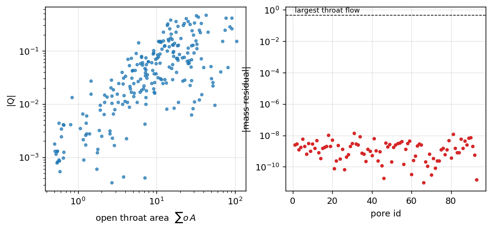
order = np.argsort(-np.abs(Q))[:5]
print(f"{'pore i':>7} {'pore j':>7} {'Q':>12} {'dp':>12} {'open area':>10}")
for t in order:
    i, j = net["throats"][t]
    print(f"{i:7d} {j:7d} {Q[t]:12.4e} {dp[t]:12.4e} {A[t]:10.1f}")
pore i pore j Q dp open area
1 2 4.7046e-01 4.8218e-03 42.5
52 57 4.5990e-01 7.2679e-03 32.0
23 28 -4.3591e-01 -8.2862e-03 34.1
37 39 -4.1189e-01 -4.3757e-04 76.5
10 15 -4.1104e-01 -4.2369e-04 90.5Reading the numbers
- Q is exact, dp is a model. The flow rates are discrete-flux identities; the pressure drops sample the pressure at two points and add the macroscopic gradient along the min-image path. On strongly constricted geometry the per-throat conductance \(g = Q/\Delta p\) is clean; on loose packings (porosity ≳ 0.6) the intra-pore viscous pressure variation rivals the throat drops and \(g\) scatters — that is a property of the point-pressure PNM abstraction, not of the extraction.
- Parallel throats are resolved. Throats are connected interface patches: two pores touching in two places (e.g. through the periodic wrap) give two entries, so the throat list can repeat a pore pair — key on the throat index.
- Both IBM variants work. With
set_ghost_projection(True)pass the sameget_ox_proj()openness; the bookkeeping is then truncation-accurate (the ghost-cell scheme is not locally conservative at walls) with the residual reporting the per-pore wall leak. - It scales. Both the extraction and the network-flow accumulation have distributed (MPI) variants on the shared block decomposition (
pnm.extract_pore_network_mpi,pnm.extract_network_flow_mpi), bit-exact to the single-rank results shown here.