# Makes this notebook run out-of-the-box on Colab/Binder. A real user just needs the
# published package; this installs it on first run. Authors can instead point at a
# local source build of the suite with the PECLET_LOCAL_BUILD env var.
import importlib.util, os, subprocess, sys
_local = os.environ.get("PECLET_LOCAL_BUILD")
if _local:
    sys.path.insert(0, _local)                                  # local source build
elif importlib.util.find_spec("peclet") is None:
subprocess.run([sys.executable, "-m", "pip", "install", "-q", "peclet"], check=True)A droplet on a wall: static contact angles on immersed solids
Set the angle, get the angle — to about a degree up to 90°, and to 2 % of the cap radius on a curved solid. Plus the one wall placement that silently freezes the contact line.
flow
vof
two-phase
wetting
IBM
verification
 Wants a GPU build: this page runs eleven \(64^3\)-class two-phase simulations.
What you’ll learn
A wetting condition is the one piece of two-phase physics that lives inside the solid. Everything else — the interface, the curvature, the surface-tension force — is a statement about the fluid; a contact angle is a statement about what the fluid’s stencils should see where there is no fluid at all. Get it wrong and the symptom is not a crash: it is a droplet that quietly settles at the wrong shape.
This page puts peclet’s static contact angle on an SDF solid through the two checks that have closed-form answers:
- A drop on a flat wall. Prescribe \(\theta\), run to rest, and read the apparent angle back off the equilibrium spherical cap. Measured 30.7° / 60.0° / 88.8° / 116.9° for \(\theta_{\text{set}} =\) 30 / 60 / 90 / 120 at 24 cells per drop diameter — within 1.2° up to 90°, and −3.1° at 120°, where the contact line itself is resolved by fewer than ten cells.
- A drop on a solid sphere. The equilibrium is a spherical cap whose sphere meets the solid sphere at \(\theta\) — a one-dimensional root solve from the conserved volume. The measured cap radius lands within 2.3 % at \(\theta = 60°/90°/120°\), and the curved wall costs nothing over the flat one.
Along the way: liquid volume conserved to \(10^{-14}\), near-wall spurious currents about an order of magnitude above the free-droplet floor, and — the finding worth the price of the page — where you place a flat SDF wall inside its cell decides whether the contact line can move at all. Put it at a half-integer coordinate and the wall cell’s tangential faces close, the contact line pins, and the unrelieved Young force shows up as a velocity of order 1.
The conclusion to carry away: the angle is imposed entirely through the colour field inside the solid — no force is added at the wall — and it is an exact fixed point of the discrete scheme. What limits the accuracy is how many cells the contact line has, not the wetting model.
The problem
A sessile drop at rest is a two-line problem. Surface tension makes the free surface a constant-curvature cap; Young’s condition makes it meet the solid at the equilibrium angle set by the three interfacial tensions,
\[ \cos\theta = \frac{\sigma_{sg} - \sigma_{sl}}{\sigma_{lg}} . \tag{1}\]
With no gravity the equilibrium of a drop of volume \(V\) on a flat wall is therefore a spherical cap: contact radius \(a\), apex height \(h\), with
\[ V = \frac{\pi h}{6}\left(3a^2 + h^2\right), \qquad \tan\frac{\theta}{2} = \frac{h}{a} . \tag{2}\]
Two measurements (\(V\) and \(h\)) give the third quantity and the angle, and this is how the angle is read back below. It matters which two: \(V\) is conserved to round-off by the geometric transport and \(h\) is a column sum of the colour field, so Equation 2 is well conditioned on a flat wall — while reading the contact radius off the first open fluid plane is biased, because that plane’s colour is an average over \(z \in [z_w, z_w + 1]\) and not the section at the wall. Both are printed below so you can see the size of the bias.
How the angle enters the discretization
peclet represents the solid by a signed distance field (\(\varphi > 0\) is fluid) and the liquid by a colour field \(C\) — the liquid fraction of each cell’s fluid volume. The geometric Weymouth–Yue transport (Weymouth and Yue 2010) moves \(C\) through cut cells with openness-weighted fluxes, and a balanced-force continuum surface force (Brackbill et al. 1992; Francois et al. 2006; Popinet 2009) turns the curvature into momentum. None of that machinery knows about wetting.
The wetting condition is imposed by filling the colour field inside the solid. Write \(\mathbf{n}_w = \nabla\varphi/|\nabla\varphi|\) for the wall normal (solid → fluid) and \(\mathbf{m}\) for the PLIC interface normal (liquid → gas). Measuring \(\theta\) through the liquid, the contact-line condition is simply
\[ \mathbf{m}\cdot\mathbf{n}_w = \cos\theta , \tag{3}\]
so \(\theta = 0\) (complete wetting) puts the interface parallel to the wall with the liquid film between it and the solid, and \(\theta = 180°\) empties the band. For each band cell inside the solid the solver walks along \(\mathbf{n}_w\) to the first fluid cell, takes the azimuth of that cell’s interface normal, builds the target normal \(\mathbf{m}_\theta = \cos\theta\,\mathbf{n}_w + \sin\theta\, \hat{\mathbf{t}}\), and writes the volume fraction of that plane into the band cell. The height-function/MYC curvature cascade — unchanged — then reads a consistent interface across the wall and returns the curvature of a surface meeting the solid at \(\theta\); the balanced force does the rest.
This is the volume-fraction form of the Afkhami–Bussmann height-function boundary condition (Afkhami and Bussmann 2008, 2009), and it is the same family as Basilisk’s embedded-boundary contact angle (Tavares et al. 2024; Popinet and Tavares 2024). Two design points are worth stating because they are what makes it work:
- The fill is exactly idempotent. The plane is anchored by matching the anchor cell’s own liquid volume, not by a geometric pivot point. An interface that already meets the wall at \(\theta\) is reproduced to \(10^{-15}\), so \(\theta\) is a genuine fixed point of the discrete scheme rather than an attractor with an offset.
- No force is added at the wall. The entire wetting model is Equation 3 expressed as cell fractions. There is nothing to balance against the CSF, and nothing that can put energy into the near-wall velocity by construction.
ImportantA run whose pressure solve hit its iteration cap is not a result
Every run on this page records last_pressure_iterations() against its cap and max_open_divergence(), and reports both. A capped solve means the projection did not converge, the velocity field is not discretely divergence-free, and the geometric transport’s conservation guarantee — which is conditional on that — no longer holds. Such runs are discarded, not quoted. (None of the runs below capped: 9–12 iterations against a cap of 300. The numbers are printed.)
import math
import numpy as np
import matplotlib.pyplot as plt
from peclet import flow

plt.rcParams.update({"figure.dpi": 130, "font.size": 10, "axes.grid": True,
                     "grid.alpha": 0.3, "axes.axisbelow": True,
                     "figure.facecolor": "white", "savefig.bbox": "tight"})
BLUE, RED, GREY, GREEN, ORANGE = "#1f77b4", "#d62728", "0.80", "#2ca02c", "#ff7f0e"
DEG = math.pi / 180.0
PRESS_CAP = 300
The scene: a cap on a slab
The wall is an SDF slab, not a single ramp. The box is periodic, so a lone wall would put a spurious fluid/solid seam at the wrap plane three cells from the band; a slab bounded at both ends keeps the wrap deep inside the solid where the distance field is continuous.
The initial condition is the exact spherical cap of the prescribed angle, sampled as volume fractions by \(4^3\) subsampling of the fluid part of each cell — because \(C\) is a fraction of the fluid volume, not of the cell. Starting at the prescribed angle makes this the fixed-point protocol: the question is whether the discrete equilibrium is the angle you asked for. (Starting from a hemisphere instead — the attraction protocol — is what the wall-placement study at the end of the page does.)
def cap_sphere(volume, theta_deg):
    """Radius and centre offset of the sphere whose cap of contact angle theta,
    resting on z = 0, has the given volume: V = pi Rc^3 (1-cos t)^2 (2+cos t)/3."""
    ct = math.cos(theta_deg * DEG)
    Rc = (3.0 * volume / (math.pi * (1.0 - ct) ** 2 * (2.0 + ct))) ** (1.0 / 3.0)
    return Rc, -Rc * ct


def cap_colour(nx, ny, nz, cx, cy, zw, R, theta_deg):
    """Liquid volume fractions of a spherical cap of contact angle theta on the wall
    z = zw, with the volume of a hemisphere of radius R. 4^3 subsampling of the FLUID
    part of each cell."""
    Rc, zc = cap_sphere(2.0 / 3.0 * math.pi * R ** 3, theta_deg)
    sub = (np.arange(4) + 0.5) / 4.0
    px = np.arange(nx)[:, None, None, None, None, None] + sub[None, None, None, :, None, None]
    py = np.arange(ny)[None, :, None, None, None, None] + sub[None, None, None, None, :, None]
    pz = np.arange(nz)[None, None, :, None, None, None] + sub[None, None, None, None, None, :]
    inside = ((px - cx) ** 2 + (py - cy) ** 2 + (pz - zw - zc) ** 2) < Rc * Rc
    fluid = np.broadcast_to(pz >= zw, inside.shape)
    tot = fluid.sum(axis=(3, 4, 5))
    return np.asfortranarray(np.where(tot > 0, (fluid & inside).sum(axis=(3, 4, 5))
                                      / np.maximum(tot, 1), 0.0).astype(float))


def slab_sdf(nx, ny, nz, zw):
    """A solid slab occupying z < zw and z > nz - zw (positive = fluid)."""
    z = (np.arange(nz) + 0.5)[None, None, :]
    return np.asfortranarray(
        np.broadcast_to(np.minimum(z - zw, (nz - zw) - z), (nx, ny, nz)).astype(float))
Driving the solver
Six calls. set_solid(..., cutcell_pressure=True) is required — the colour transport weights every flux by the face openness, and the staircase pressure operator has none, so the solver raises if you ask for VoF through a staircase solid. set_contact_angle(theta) is the whole wetting model.
Surface tension is explicit, so the time step is capped by the Brackbill capillary limit capillary_dt(); on top of that the geometric transport wants an interface-local Courant number below about 0.2, and in cut cells that limiter is tighter than the plain one by up to \(1/\varepsilon\). The driver below tracks both.
We use \(\mathrm{Oh} = \mu/\sqrt{\rho\sigma D} = 0.1\), which is the fastest relaxation the capillary time step allows without ringing.
def maxvel(s, zlo=None):
    m = 0.0
    for f in (s.get_u, s.get_v, s.get_w):
        v = np.abs(f())
        m = max(m, float(v.max()) if zlo is None else float(v[:, :, zlo:].max()))
    return m


def relax(s, steps, cfl=0.15, probe=25):
    """Run to rest with dt under both the capillary and the interface-CFL limits."""
    dt_cap = 0.5 * s.capillary_dt()
    dt = dt_cap
    s.set_dt(dt)
    iters, capped, div, trace = 0, 0, 0.0, []
    for i in range(steps):
        c = s.vof_max_courant()
        if c > cfl:
            dt = min(dt_cap, dt * cfl / c); s.set_dt(dt)
        elif dt < dt_cap and c < 0.5 * cfl:
            dt = min(dt_cap, 1.2 * dt); s.set_dt(dt)
        s.step()
        it = s.last_pressure_iterations()
        iters = max(iters, it)
        capped += it >= PRESS_CAP                 # rule: a capped solve invalidates the run
        div = max(div, s.max_open_divergence())   # the conservation floor
        if (i + 1) % probe == 0:
            trace.append((i + 1, maxvel(s)))
    return dict(dt=dt, iters=iters, capped=capped, div=div, trace=np.array(trace))


def drop_on_wall(theta, ratio=1.0, steps=500, R=12.0, nx=64, nz=40, zw=4.25,
                 sigma=1.0, oh=0.1, theta_init=None):
    """A liquid cap on a flat SDF wall at z = zw, relaxed at contact angle `theta`."""
    mu = oh * math.sqrt(1.0 * sigma * 2.0 * R)
    s = flow.Solver(nx, nx, nz)
    s.set_rho(1.0)
    s.set_mu(mu)
    s.set_solid(slab_sdf(nx, nx, nz, zw), cutcell_pressure=True)
    s.enable_vof()
    if ratio != 1.0:                                   # two-phase closures of the colour
        s.set_property_model("rho", "linear", "C", [1.0 / ratio, 1.0 - 1.0 / ratio])
        s.set_property_model("mu", "linear", "C", [mu / ratio, mu - mu / ratio])
    s.set_vof(cap_colour(nx, nx, nz, nx / 2, nx / 2, zw, R,
                         theta if theta_init is None else theta_init))
    s.set_surface_tension(sigma)
    s.set_contact_angle(theta)                         # <- the entire wetting model

    V0 = s.vof_diagnostics()["volume"]
    r = relax(s, steps)

    d, cd = s.vof_diagnostics(), s.contact_angle_diagnostics()
    C, eps = s.get_vof(), s.vof_geometry(0)            # colour and cell fluid fraction
    ix = nx // 2
    h = float((C[ix, ix, :] * eps[ix, ix, :]).sum())   # apex height: the colour column
    V = d["volume"]
    a = math.sqrt(max((6.0 * V / (math.pi * h) - h * h) / 3.0, 1e-12))     # @eq-cap
    z0 = int(math.ceil(zw))
    a_contour = math.sqrt(float(C[:, :, z0].sum()) / math.pi)              # the biased read
    kw = int(math.floor(zw))                           # the wall-adjacent cut cell
    r.update(theta_set=theta, theta=2 * math.degrees(math.atan2(h, a)), h=h, a=a,
             theta_contour=2 * math.degrees(math.atan2(h, a_contour)), a_contour=a_contour,
             dV=abs(V - V0) / V0, volume=V, mu=mu, sigma=sigma, ratio=ratio,
             Ca_open=mu * maxvel(s, z0 + 1) / sigma, umax=maxvel(s),
             apparent=cd["mean_apparent_angle"], solid_sum=d["solid_sum"],
             band=(cd["contact_cells"], cd["neighbour_cells"], cd["pure_cells"]),
             C=C, eps=eps, zw=zw, nx=nx, nz=nz, R=R,
             eps_wall=float(eps[ix, ix, kw]), ox_wall=float(s.get_ox()[ix, ix, kw]))
    return r
1. A drop on a flat wall
Four angles, 500 capillary-limited steps each, \(D/\Delta = 24\) in a \(64\times64\times40\) box, matched fluids. The wall sits at \(z = 4.25\) — a quarter-integer, for a reason the last section of this page measures.
THETAS = [30.0, 60.0, 90.0, 120.0]
flat = {th: drop_on_wall(th) for th in THETAS}

print(f"{'theta_set':>9} {'theta':>8} {'err':>7} {'h':>7} {'a':>7} {'contour th':>11} "
      f"{'dV/V':>9} {'Ca(open)':>10} {'max|u|':>9} {'iters':>8} {'max|div|':>9}")
for th, r in flat.items():
    print(f"{th:9.0f} {r['theta']:8.3f} {r['theta']-th:+7.3f} {r['h']:7.3f} {r['a']:7.3f} "
          f"{r['theta_contour']:11.3f} {r['dV']:9.1e} {r['Ca_open']:10.2e} {r['umax']:9.2e} "
          f"{r['iters']:5d}/{PRESS_CAP} {r['div']:9.1e}")
WORST = max(abs(r["theta"] - th) for th, r in flat.items())
print(f"\nworst |theta - theta_set| over the sweep: {WORST:.2f} deg")
print(f"worst below 90 deg:                       "
      f"{max(abs(flat[t]['theta'] - t) for t in (30.0, 60.0, 90.0)):.2f} deg")
theta_set theta err h a contour th dV/V Ca(open) max|u| iters max|div|
30 30.688 +0.688 5.532 20.161 34.474 1.7e-14 2.96e-04 1.45e-03 9/300 1.8e-12
60 59.980 -0.020 8.839 15.316 62.765 3.3e-15 3.68e-04 2.09e-03 10/300 3.0e-12
90 88.841 -1.159 11.880 12.123 89.399 5.0e-16 2.20e-04 4.50e-04 11/300 3.6e-13
120 116.858 -3.142 14.798 9.094 114.079 2.6e-15 7.99e-04 1.82e-03 10/300 1.5e-12
worst |theta - theta_set| over the sweep: 3.14 deg
worst below 90 deg: 1.16 degThe measured equilibria are 30.7° / 60.0° / 88.8° / 116.9° against the prescribed 30° / 60° / 90° / 120°. Three of the four rows are inside 1.2°; the 120° row is -3.1° low, which the “resolution and limits” section below traces to the contact radius rather than to the wetting model.
Note the two independent readings of the angle in the table. The volume-consistent one (Equation 2) and the first-fluid-plane contour agree to under a degree at 90° and part company by 3.8° at 30° — the flatter the cap, the more the near-wall averaging biases a contour read. That gap is a measurement artefact, and it is worth knowing before comparing any code’s contact angle with any other’s.
fig, axes = plt.subplots(1, 4, figsize=(9.6, 2.9), sharey=True)
for ax, th in zip(axes, THETAS):
    r = flat[th]
    nx, nz, zw = r["nx"], r["nz"], r["zw"]
    x = np.arange(nx) + 0.5
    z = np.arange(nz) + 0.5
    ax.contour(x, z, r["C"][:, nx // 2, :].T, levels=[0.5], colors=[BLUE], linewidths=1.8)
    Rc, zc = cap_sphere(r["volume"], th)                 # the reference cap
    t = np.linspace(0, 2 * np.pi, 400)
    cx, cz = nx / 2 + Rc * np.cos(t), zw + zc + Rc * np.sin(t)
    keep = cz >= zw
    ax.plot(cx[keep], cz[keep], "--", color=RED, lw=1.3)
    ax.axhspan(0, zw, color="0.75", zorder=0)
    ax.axhline(zw, color="0.35", lw=1.0)
    ax.set(xlim=(nx / 2 - 24, nx / 2 + 24), ylim=(0, 34), aspect="equal",
           title=f"$\\theta_{{set}} = {th:.0f}°$\nmeasured {r['theta']:.1f}°")
    ax.set_xlabel("x  [cells]")
    ax.grid(alpha=0.2)
axes[0].set_ylabel("z  [cells]")
axes[0].plot([], [], color=BLUE, lw=1.8, label=r"$C=\frac{1}{2}$ (measured)")
axes[0].plot([], [], "--", color=RED, lw=1.3, label="exact cap")
axes[0].legend(fontsize=7, loc="upper left", framealpha=0.9)
plt.show()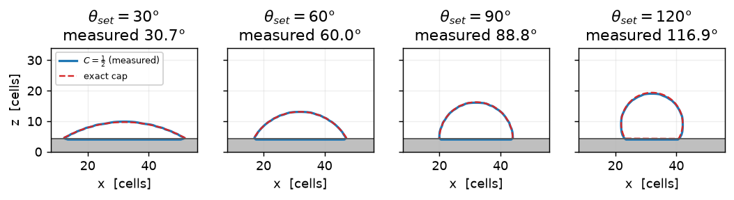
2. The same sweep at density ratio 100
Matched fluids isolate the wetting model; a real drop does not have them. The density and viscosity become linear closures of the colour, which is what switches the solver onto its variable-density projection, and everything else is identical.
flat100 = {th: drop_on_wall(th, ratio=100.0) for th in THETAS}

print(f"{'theta_set':>9} {'ratio 1':>9} {'ratio 100':>11} {'difference':>12} "
      f"{'dV/V':>9} {'Ca(open)':>10} {'iters':>9} {'max|div|':>9}")
for th in THETAS:
    a, b = flat[th]["theta"], flat100[th]["theta"]
    print(f"{th:9.0f} {a:9.3f} {b:11.3f} {b-a:+12.3f} {flat100[th]['dV']:9.1e} "
          f"{flat100[th]['Ca_open']:10.2e} {flat100[th]['iters']:6d}/{PRESS_CAP} "
          f"{flat100[th]['div']:9.1e}")
DRIFT100 = max(abs(flat100[t]["theta"] - flat[t]["theta"]) for t in THETAS)
print(f"\nlargest ratio-1 vs ratio-100 difference: {DRIFT100:.2f} deg")
theta_set ratio 1 ratio 100 difference dV/V Ca(open) iters max|div|
30 30.688 29.920 -0.768 3.2e-12 1.72e-03 11/300 8.5e-09
60 59.980 58.360 -1.620 1.9e-11 2.57e-03 11/300 1.4e-08
90 88.841 88.439 -0.402 2.5e-11 3.02e-03 11/300 2.0e-08
120 116.858 116.415 -0.443 1.5e-12 4.48e-03 12/300 2.3e-08
largest ratio-1 vs ratio-100 difference: 1.62 degfig, ax = plt.subplots(figsize=(4.8, 4.2))
tt = np.array([20, 132])
ax.fill_between(tt, tt - 3, tt + 3, color=BLUE, alpha=0.13, lw=0, label="±3° gate band")
ax.plot(tt, tt, color="0.4", lw=1.0, label="ideal")
ax.plot(THETAS, [flat[t]["theta"] for t in THETAS], "o-", color=BLUE, ms=7, lw=1.6,
label="density ratio 1")
ax.plot(THETAS, [flat100[t]["theta"] for t in THETAS], "s--", color=ORANGE, ms=6, lw=1.4,
label="density ratio 100")
ax.set(xlabel=r"prescribed $\theta$ [deg]", ylabel=r"measured apparent $\theta$ [deg]",
xlim=(20, 132), ylim=(20, 132), title="The angle you set is the angle you get")
ax.set_aspect("equal")
ax.legend(fontsize=8, loc="upper left")
plt.show()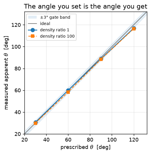
At a hundredfold density contrast the equilibrium angles move by at most 1.6° and the residual at 120° is the same −3.6°. That is the check that matters for the model: the fill is a purely geometric statement about the colour field, and the measurement confirms it does not inherit anything from the momentum equation it feeds.
3. The approach to rest
The fixed-point protocol starts at equilibrium, so what the velocity trace shows is the relaxation of the discrete transient — the initial condition is an exact cap, but the discrete curvature of an exact cap is not exactly constant, and the band fill has to settle into the shape it is idempotent on.
fig, ax = plt.subplots(figsize=(5.2, 3.6))
cols = {30.0: BLUE, 60.0: GREEN, 90.0: ORANGE, 120.0: RED}
for th in THETAS:
    tr = flat[th]["trace"]
    ax.semilogy(tr[:, 0], tr[:, 1], color=cols[th], lw=1.6, label=f"$\\theta = {th:.0f}°$")
ax.set(xlabel="step", ylabel=r"$\max|\mathbf{u}|$",
       title="Relaxation to the equilibrium cap ($D/\\Delta = 24$, Oh $= 0.1$)")
ax.legend(fontsize=8, ncol=2)
plt.show()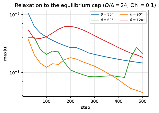
4. A drop on a solid sphere
A flat wall lets the fill get away with a lot: \(\mathbf{n}_w\) is constant, the band is three flat rows, and every column sees the same geometry. A curved solid is the real test, and it also has a closed-form answer.
Put a drop of volume \(V\) on a solid sphere of radius \(R_s\). At rest the free surface is a sphere of radius \(R_c\) whose centre sits a distance \(d\) from the solid’s, and the two spheres must meet at \(\theta\) — which by the law of cosines is
\[ d^2 = R_s^2 + R_c^2 - 2 R_s R_c \cos\theta , \tag{4}\]
while the liquid volume is the drop sphere minus the lens the two spheres share. Given \((V, \theta)\) that is a one-dimensional root solve for \(R_c\) — the reference shape, with no fitting and no free parameters.
def lens_volume(Rs, Rc, d):
    """Volume of the intersection of spheres (centre 0, radius Rs) and (centre d, Rc)."""
    if d >= Rs + Rc:
        return 0.0
    if d <= abs(Rs - Rc):
        return 4.0 / 3.0 * math.pi * min(Rs, Rc) ** 3
    return (math.pi * (Rs + Rc - d) ** 2
            * (d * d + 2 * d * Rc - 3 * Rc ** 2 + 2 * d * Rs + 6 * Rc * Rs - 3 * Rs ** 2)
            / (12.0 * d))


def drop_volume(Rs, Rc, d):
    return 4.0 / 3.0 * math.pi * Rc ** 3 - lens_volume(Rs, Rc, d)


def cap_from_volume(Rs, V, theta_deg):
    """(V, theta) -> the reference cap sphere (Rc, d) via @eq-lawcos. Bisection."""
    ct = math.cos(theta_deg * DEG)
    lo, hi = 1e-3, 50.0 * Rs
    for _ in range(200):
        mid = 0.5 * (lo + hi)
        d = math.sqrt(max(Rs ** 2 + mid ** 2 - 2 * Rs * mid * ct, 0.0))
        (lo, hi) = (mid, hi) if drop_volume(Rs, mid, d) < V else (lo, mid)
    Rc = 0.5 * (lo + hi)
    return Rc, math.sqrt(max(Rs ** 2 + Rc ** 2 - 2 * Rs * Rc * ct, 0.0))


def theta_from_volume_apex(Rs, V, H):
    """The inverse reading: (V, apex height H = d + Rc) -> (Rc, d, theta)."""
    lo, hi = 1e-3, H
    for _ in range(200):
        Rc = 0.5 * (lo + hi)
        (lo, hi) = (Rc, hi) if drop_volume(Rs, Rc, max(H - Rc, 0.0)) < V else (lo, Rc)
    Rc = 0.5 * (lo + hi)
    d = H - Rc
    ct = (Rs ** 2 - d ** 2 + Rc ** 2) / (2.0 * Rs * Rc)
    return Rc, d, math.degrees(math.acos(max(-1.0, min(1.0, ct))))
def drop_on_sphere(theta, steps=500, Rs=12.0, Rd=8.0, n=64, sigma=1.0, oh=0.1):
"""A drop with the volume of a sphere of radius Rd, resting on a solid sphere Rs."""
mu = oh * math.sqrt(1.0 * sigma * 2.0 * Rd)
c = n * 0.5
ax_ = (np.arange(n) + 0.5)
sdf = np.asfortranarray(np.sqrt((ax_[:, None, None] - c) ** 2
+ (ax_[None, :, None] - c) ** 2
+ (ax_[None, None, :] - c) ** 2) - Rs)
V = 4.0 / 3.0 * math.pi * Rd ** 3
Rc0, d0 = cap_from_volume(Rs, V, theta)
sub = (np.arange(4) + 0.5) / 4.0 # exact-ish initial fractions
px = np.arange(n)[:, None, None, None, None, None] + sub[None, None, None, :, None, None]
py = np.arange(n)[None, :, None, None, None, None] + sub[None, None, None, None, :, None]
pz = np.arange(n)[None, None, :, None, None, None] + sub[None, None, None, None, None, :]
fluid = ((px - c) ** 2 + (py - c) ** 2 + (pz - c) ** 2) > Rs ** 2
liq = fluid & (((px - c) ** 2 + (py - c) ** 2 + (pz - c - d0) ** 2) < Rc0 ** 2)
tot = fluid.sum(axis=(3, 4, 5))
C0 = np.asfortranarray(np.where(tot > 0, liq.sum(axis=(3, 4, 5)) / np.maximum(tot, 1),
0.0).astype(float))
s = flow.Solver(n, n, n)
s.set_rho(1.0)
s.set_mu(mu)
s.set_solid(sdf, cutcell_pressure=True)
s.enable_vof()
s.set_vof(C0)
s.set_surface_tension(sigma)
s.set_contact_angle(theta)
V0 = s.vof_diagnostics()["volume"]
r = relax(s, steps)
d, cd = s.vof_diagnostics(), s.contact_angle_diagnostics()
C, eps = s.get_vof(), s.vof_geometry(0)
i = int(c)
H = float((C[i, i, :] * eps[i, i, :])[int(c):].sum()) + Rs # apex above the centre
Vm = d["volume"]
Rc, dd, th = theta_from_volume_apex(Rs, Vm, H)
r.update(theta_set=theta, theta=th, Rc=Rc, Rc_ref=Rc0, d=dd, d_ref=d0, H=H,
H_ref=d0 + Rc0, dV=abs(Vm - V0) / V0, Ca=mu * maxvel(s) / sigma,
apparent=cd["mean_apparent_angle"], solid_sum=d["solid_sum"],
C=C, n=n, Rs=Rs, c=c, mu=mu)
return r
SPH_THETAS = [60.0, 90.0, 120.0]
sph = {th: drop_on_sphere(th) for th in SPH_THETAS}
print(f"{'theta_set':>9} {'Rc':>7} {'Rc ref':>8} {'Rc err':>9} {'H':>7} {'H ref':>7} "
f"{'theta(V,H)':>11} {'local th':>9} {'dV/V':>9} {'iters':>9}")
for th, r in sph.items():
print(f"{th:9.0f} {r['Rc']:7.3f} {r['Rc_ref']:8.3f} "
f"{100*(r['Rc']-r['Rc_ref'])/r['Rc_ref']:+8.2f}% {r['H']:7.3f} {r['H_ref']:7.3f} "
f"{r['theta']:11.2f} {r['apparent']:9.2f} {r['dV']:9.1e} "
f"{r['iters']:6d}/{PRESS_CAP}")
RC_WORST = max(abs(r["Rc"] - r["Rc_ref"]) / r["Rc_ref"] for r in sph.values())
print(f"\nworst cap-radius error: {100*RC_WORST:.2f} %")theta_set Rc Rc ref Rc err H H ref theta(V,H) local th dV/V iters
60 9.368 9.585 -2.27% 21.041 20.578 64.86 74.38 4.4e-11 9/300
90 8.612 8.549 +0.74% 23.067 23.283 87.44 89.43 2.2e-11 9/300
120 8.174 8.119 +0.68% 25.178 25.649 113.53 113.92 1.1e-11 9/300
worst cap-radius error: 2.27 %fig, axes = plt.subplots(1, 3, figsize=(8.4, 3.2), sharey=True)
t = np.linspace(0, 2 * np.pi, 500)
for ax, th in zip(axes, SPH_THETAS):
r = sph[th]
n, c, Rs = r["n"], r["c"], r["Rs"]
g = np.arange(n) + 0.5
ax.contour(g, g, r["C"][:, int(c), :].T, levels=[0.5], colors=[BLUE], linewidths=1.8)
ax.plot(c + r["Rc_ref"] * np.cos(t), c + r["d_ref"] + r["Rc_ref"] * np.sin(t),
"--", color=RED, lw=1.3)
ax.add_patch(plt.Circle((c, c), Rs, color="0.75", zorder=0))
ax.plot(c + Rs * np.cos(t), c + Rs * np.sin(t), color="0.35", lw=1.0)
ax.set(xlim=(c - 20, c + 20), ylim=(c - 16, c + 26), aspect="equal",
title=f"$\\theta_{{set}} = {th:.0f}°$\n$R_c$ "
f"{100*(r['Rc']-r['Rc_ref'])/r['Rc_ref']:+.2f} %")
ax.set_xlabel("x [cells]")
ax.grid(alpha=0.2)
axes[0].set_ylabel("z [cells]")
axes[0].plot([], [], color=BLUE, lw=1.8, label=r"$C=\frac{1}{2}$")
axes[0].plot([], [], "--", color=RED, lw=1.3, label="analytic cap")
axes[0].legend(fontsize=7, loc="lower left", framealpha=0.9)
plt.show()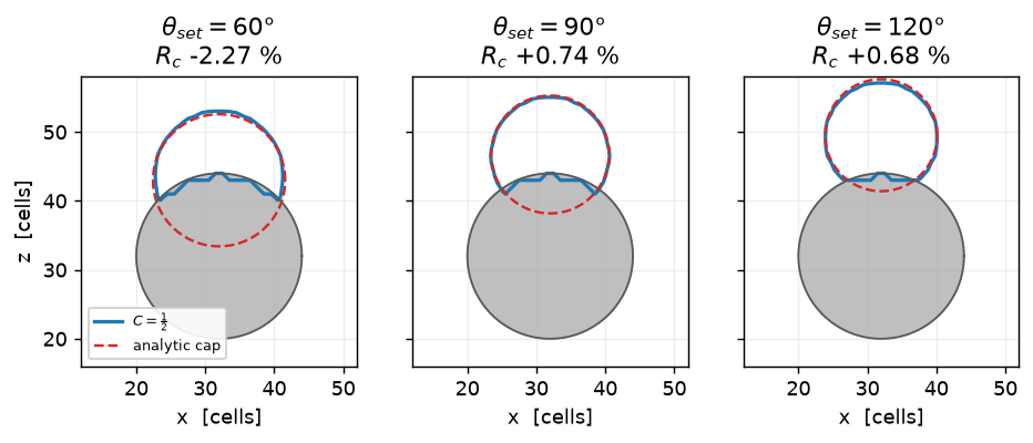
The measured cap radii are within 2.3 % of the analytic two-sphere solution at all three angles — on a wall whose normal turns from column to column, which is the case the flat wall cannot exercise.
NoteWhy the table gates the cap radius and not the angle
The angle column of the sphere table is off by up to 6.5° while the shape is right to under a percent, and that is a statement about the measurement. The angle is inferred by inverting \((V, H) \to (R_c, d) \to \theta\) from the conserved volume and the apex height, and that inversion is badly conditioned: here \(\mathrm{d}\theta/\mathrm{d}H \approx 10°\) per cell, so a half-cell error in a colour column sum — exactly what an interface crossing a cell diagonally gives — is worth five degrees. The cap radius is the well-conditioned reading, and the solver’s local estimator (contact_angle_diagnostics()['mean_apparent_angle'], the last column of the table) is the other one: it reads 74° / 89° / 114° against the prescribed 60 / 90 / 120. Global-shape inversions are a trap in wetting benchmarks generally, not just here.
5. Volume, and what a contact line costs in spurious currents
Two health numbers. The liquid volume must be conserved by the geometric transport to the projection’s own divergence residual — that is the whole point of a Weymouth–Yue scheme, and the openness-weighted cut-cell form keeps it. And the spurious currents near a contact line are the honest price of the wetting model: the parasitic-currents page measures \(\mathrm{Ca} = 2.6\times10^{-5}\) for a free droplet at the same \(D/\Delta\), which is the floor a wetting run can be compared against.
CA_FREE = 2.6e-5      # free droplet at D/dx = 24, from the parasitic-currents page
print(f"{'':<14}{'theta':>7} {'dV/V':>10} {'max|div|':>10} {'Ca(open fluid)':>16} "
      f"{'x free droplet':>16} {'solid colour':>13}")
for tag, tab in (("flat, ratio 1", flat), ("flat, ratio 100", flat100)):
    for th in THETAS:
        r = tab[th]
        print(f"{tag if th == THETAS[0] else '':<14}{th:7.0f} {r['dV']:10.1e} "
              f"{r['div']:10.1e} {r['Ca_open']:16.2e} "
              f"{r['Ca_open']/CA_FREE:15.0f}x {r['solid_sum']:13.1e}")
for th in SPH_THETAS:
    r = sph[th]
    print(f"{'sphere' if th == SPH_THETAS[0] else '':<14}{th:7.0f} {r['dV']:10.1e} "
          f"{r['div']:10.1e} {r['Ca']:16.2e} {r['Ca']/CA_FREE:15.0f}x "
          f"{r['solid_sum']:13.1e}")

CA_RANGE = (min(flat[t]["Ca_open"] for t in THETAS), max(flat[t]["Ca_open"] for t in THETAS))
DV_MAX = max(flat[t]["dV"] for t in THETAS)
print(f"\nflat wall, ratio 1: dV/V <= {DV_MAX:.1e};  Ca in "
      f"[{CA_RANGE[0]:.1e}, {CA_RANGE[1]:.1e}] = "
      f"{CA_RANGE[0]/CA_FREE:.0f}x .. {CA_RANGE[1]/CA_FREE:.0f}x the free droplet")
theta dV/V max|div| Ca(open fluid) x free droplet solid colour
flat, ratio 1 30 1.7e-14 1.8e-12 2.96e-04 11x 0.0e+00
60 3.3e-15 3.0e-12 3.68e-04 14x 0.0e+00
90 5.0e-16 3.6e-13 2.20e-04 8x 0.0e+00
120 2.6e-15 1.5e-12 7.99e-04 31x 0.0e+00
flat, ratio 100 30 3.2e-12 8.5e-09 1.72e-03 66x 0.0e+00
60 1.9e-11 1.4e-08 2.57e-03 99x 0.0e+00
90 2.5e-11 2.0e-08 3.02e-03 116x 0.0e+00
120 1.5e-12 2.3e-08 4.48e-03 172x 0.0e+00
sphere 60 4.4e-11 1.1e-08 1.25e-03 48x 0.0e+00
90 2.2e-11 9.8e-09 3.33e-03 128x 0.0e+00
120 1.1e-11 6.5e-09 1.15e-03 44x 0.0e+00
flat wall, ratio 1: dV/V <= 1.7e-14; Ca in [2.2e-04, 8.0e-04] = 8x .. 31x the free dropletThree things to read off that table.
Volume is exact. On the flat wall the drift is at most 1.7e-14 relative over 500 steps, and the colour inside the solid is exactly zero in every run — the transport never leaks liquid into the wall, and the band fill the stencils read is a separate working field.
The conservation floor is the pressure solve, not the advection. The matched-fluid flat-wall runs carry max|div(open·u)| around \(10^{-12}\) and drift at \(10^{-14}\); the harder projections — the variable-density rows and the curved solid — carry \(10^{-8}\) and drift at \(10^{-11}\). The ratio of the two is the same everywhere, which is the signature of a transport whose conservation is exact and inherits the projection’s residual. If you need tighter volume conservation, tighten the projection; refining the transport will not help.
A contact line costs about an order of magnitude in spurious currents. With matched fluids the near-wall \(\mathrm{Ca}\) over the open fluid runs 2.2e-04–8.0e-04, i.e. 8–31× the free-droplet floor; at density ratio 100 the same measurement is five to fourteen times larger again. This is measured over the open fluid only (\(z\) above the first fully open plane). Velocities on the immersed DOFs inside and on the wall are constrained by the IBM and multiplied by zero openness everywhere they could act; quoting them would measure the immersed boundary rather than the surface-tension balance — and, as the next section shows, at one particular wall placement they are enormous while the physics is unchanged.
6. Resolution and limits — read this before using it
This rung is honest about four things.
The contact line needs about ten cells
The error over the sweep is monotone in \(\theta\): +0.7 / -0.0 / -1.2 / -3.1 degrees at 30 / 60 / 90 / 120. So is the contact radius: 20.2 / 15.3 / 12.1 / 9.1 cells. The row that misses is the row whose contact line is resolved by fewer than ten radial cells, and at \(\theta = 150°\) on this grid the contact radius would be about 5 cells, where the solver’s own study measures −3.8°.
The practical rule: size the grid on the contact radius \(a\), not on the drop diameter. For an obtuse angle \(a \ll D\), so a \(D/\Delta\) that is generous for a free droplet is not generous for a wetting one.
The residual above 90° is converged, and unexplained
The −3.6° at 120° is not an unfinished transient. Run to rest in the solver’s own study (1500 steps, max|u| down to \(1.8\times10^{-4}\)) the same scene settles at 116.40°, and the velocity trace on this page is already flat at 500 steps. Two candidate mechanisms have been ruled out by measurement: it is not the density contrast (the ratio-100 column above reproduces it), and it is not the cut-cell reconstruction — with the wall on a cell face, where the anchor cell is uncut and that approximation is exactly absent, the same run reads worse (115.3° after 750 steps). It tracks the contact-line resolution, which is why the recommendation above is a resolution rule rather than a correction factor. The refinement that is not implemented is the solid-clipped flux polygon (Chen et al. 2025): peclet reconstructs the PLIC plane on the whole unit cell and multiplies its slab volume by the open face area, rather than clipping it against the solid as well.
It is a static angle
\(\theta\) is a per-cell field and the fill is evaluated every step, but the value it is given does not depend on the contact-line velocity. There is no dynamic contact angle and no hysteresis: an advancing and a receding contact line are given the same \(\theta\). That is rung V6 of the VoF campaign; when it lands, only what fills the \(\theta\) field changes, not the machinery on this page.
A consequence worth budgeting for: the approach to a prescribed angle is slow. The driving force vanishes as the contact line arrives, so a relaxation that has to move the line through 30° takes \(O(10^3)\) capillary-limited steps, not \(O(10^2)\) — the wall-placement run below starts from a hemisphere and is still travelling after 300.
The wall placement trap
WarningDo not put a flat SDF wall at a half-integer coordinate
It is the natural choice — it makes the wall cells “genuinely cut” — and it silently freezes the contact line. Use a quarter-integer, or put the wall exactly on a cell face.
At exactly \(z = k + \tfrac12\) the tangential MAC faces of the wall-adjacent cell sit on the SDF zero level. The openness builder treats \(\varphi > 0\) as fluid, so \(\varphi = 0\) closes them: the cell reads a fluid fraction of 0.5 and a tangential face openness of 0.000 at the same time. It is a fluid cell that can exchange nothing along the wall — no colour, no momentum — so the contact line cannot move, and the unrelieved Young force appears as a velocity of order 1 on DOFs the projection never sees.
One angle, one initial condition (a hemisphere, so the contact line has to travel), everything identical except where the wall sits inside its cell:
place = {zw: drop_on_wall(60.0, steps=300, zw=zw, theta_init=90.0) for zw in (4.25, 3.5)}
print(f"{'wall z':>7} {'eps (wall cell)':>16} {'tangential ox':>15} "
      f"{'theta @300':>11} {'max|u|':>10} {'verdict':>18}")
for zw, r in place.items():
    verdict = "mobile, cut" if r["ox_wall"] > 0 else "PINNED"
    print(f"{zw:7.2f} {r['eps_wall']:16.3f} {r['ox_wall']:15.3f} {r['theta']:11.2f} "
          f"{r['umax']:10.2e} {verdict:>18}")
UFAC = place[3.5]["umax"] / place[4.25]["umax"]
print(f"\nsame physics, same theta, same steps: max|u| differs by a factor {UFAC:.0f}")
wall z eps (wall cell) tangential ox theta @300 max|u| verdict
4.25 0.750 0.750 73.85 2.90e-02 mobile, cut
3.50 0.500 0.000 81.42 1.05e+00 PINNED
same physics, same theta, same steps: max|u| differs by a factor 36fig, (ax, axb) = plt.subplots(1, 2, figsize=(8.4, 3.3),
gridspec_kw=dict(width_ratios=[1.25, 1]))
for zw, col, lab in ((4.25, BLUE, "wall at $z = 4.25$ (quarter cell)"),
(3.5, RED, "wall at $z = 3.50$ (half cell)")):
tr = place[zw]["trace"]
ax.semilogy(tr[:, 0], tr[:, 1], color=col, lw=1.8, label=lab)
ax.set(xlabel="step", ylabel=r"$\max|\mathbf{u}|$",
title="Where the wall sits inside its cell")
ax.legend(fontsize=8, loc="center right")
x = np.arange(place[4.25]["nx"]) + 0.5
for zw, col in ((4.25, BLUE), (3.5, RED)):
r = place[zw]
z = np.arange(r["nz"]) + 0.5
axb.contour(x, z, r["C"][:, r["nx"] // 2, :].T, levels=[0.5], colors=[col],
linewidths=1.8)
axb.axhline(zw, color=col, lw=0.9, ls=":")
axb.axhspan(0, 4.25, color="0.85", zorder=0)
axb.set(xlim=(32 - 22, 32 + 22), ylim=(0, 26), aspect="equal", xlabel="x [cells]",
ylabel="z [cells]",
title=f"shape after 300 steps\n({place[4.25]['theta']:.0f}° travelling vs "
f"{place[3.5]['theta']:.0f}° stalled)")
axb.grid(alpha=0.2)
plt.show()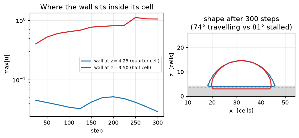
The mobile run has travelled from 90° to 74° and is still going; the pinned one sits at 81° with a max|u| of 1.05, a factor 36 larger. Neither run touched the pressure cap, both conserve volume, and there is no error message: the only visible symptom is a drop that stops at the wrong shape.
NoteA domain-BC wall is not a wetting wall
set_domain_bc(face, 1) gives a no-slip domain wall, and it does not receive the contact-angle fill — the band fill runs on the SDF classification only, so a domain wall keeps the zero-gradient (90°) colour extrapolation whatever set_contact_angle says. Model a wetting wall as an SDF slab, which is what every run on this page does.
Collocated cross-check
peclet also ships a cell-centred/collocated grid (flow.SolverColocated), and since rung V8 (2026-09-02) it runs two-phase flow: variable density in the approximate (ABC) projection, surface tension as a face acceleration, and the colour advected by the projected face field. The parasitic currents and capillary oscillations pages carry that column.
This page is not one of them, and the reason is the solid. Rung V8 is all-fluid: the cut-cell colour transport of rung V5a — openness-weighted geometric fluxes, the solid-band fill, and with it the contact-angle plane this whole page is about — exists on the staggered grid only. The composition is refused rather than silently approximated:
s = flow.SolverColocated(32, 32, 24)
s.set_rho(1.0)
s.set_mu(0.1)
s.set_solid(slab_sdf(32, 32, 24, 4.25), cutcell_pressure=True)   # accepted: single-phase is fine
try:
    s.enable_vof()
    print("enable_vof() succeeded — this page's setup would run")
except RuntimeError as e:
    print(f"enable_vof() raised RuntimeError:\n  {e}")
enable_vof() raised RuntimeError:
enable_vof: geometric VoF on SolverColocated (rung V8) is ALL-FLUID only — an immersed solid needs the cut-cell face acceleration and the matching one-sided closures, which is a later rung. Use the staggered Solver (rung V5a supports cut cells).The reverse call order is guarded in the same place rather than in set_solid: enable_vof() first and set_solid() second is accepted, and the throw then arrives from set_vof, set_surface_tension and step() with the same message. set_contact_angle itself never raises — it only records the angle — so the guard you will actually meet is the one above.
There is nothing to report here yet, and nothing to approximate: every number on this page is a staggered number, and the contact-angle model has no collocated column until the cut-cell face acceleration lands. The rising bubble page states the other half of the current rating — collocated two-phase flow is honest to density ratio \(\lesssim 100\) for cases with motion, because momentum-consistent transport is staggered-only as well.
Adapt this yourself
- Pattern the wettability.
set_contact_angle_field(theta_deg_array)takes a per-cell angle, so a chemically striped or patchy surface is one array away. The fill is evaluated per band cell, so nothing else changes. - Put it on a packing. The wall here is a slab and a sphere; the same three calls work on any SDF, including a
dem-generated sphere packing — that is the trickle-flow example, and the only extra ingredients are two-phase inflow and outflow boundaries. - Check the fill you are getting.
vof_filled_colour()returns the working colour field including the band inside the solid, andcontact_angle_diagnostics()returns the census of which rule filled each band cell (contact_cells= the θ-plane rule,neighbour_cells= averaged from mixed neighbours,pure_cells= pure-phase continuation) plus the mean locally measured apparent angle. Ifcontact_cellsis zero, your contact line is not where you think it is. - Ablate the anchor.
set_contact_angle_pivot(0..3)switches the plane’s anchor between the shipped volume-matched one and three geometric alternatives, one of which is the obvious “project the interface centroid onto the wall”. It is not idempotent — the prescribed angle stops being a fixed point — and the ablation shows by how much. - Go multi-rank. The identical script runs under
mpirun -np N python …. The band fill is built on the inner region and exchanged rather than guessed at depth, so the filled colour is bitwise decomposition-independent even when the block cut goes through the contact line.
Reproduce this
The compiled solver runs this, so its outputs are frozen into the site. To regenerate:
pip install peclet            # the solver, from PyPI
quarto render examples/droplet-wetting/index.qmd --execute
# ...or against a local source build of the suite (GPU):
PECLET_LOCAL_BUILD=/path/to/suite/flow/build_cuda OMP_NUM_THREADS=8 OMP_PROC_BIND=false \
  quarto render examples/droplet-wetting/index.qmd --execute
The same battery lives inside the solver repo as tests/study/vof_wetting.py (g1 the flat-wall sweep, g1w the wall-placement study, g2 the drop on a sphere, g4 a capillary-rise case that does not yet pass and is documented as such), and the kernel-level gates — the flat-wall idempotence of the fill to \(10^{-15}\), the rotation, the wetting limits at \(\theta = 0\) and \(180°\) — run in the vof_wetting ctest, with its MPI twin at np = 1/2/4.
References
Afkhami, S., and M. Bussmann. 2008. “Height Functions for Applying Contact Angles to 2D VOF Simulations.” International Journal for Numerical Methods in Fluids 57 (4): 453–72. https://doi.org/10.1002/fld.1651.
Afkhami, S., and M. Bussmann. 2009. “Height Functions for Applying Contact Angles to 3D VOF Simulations.” International Journal for Numerical Methods in Fluids 61 (8): 827–47. https://doi.org/10.1002/fld.1974.
Brackbill, J. U., D. B. Kothe, and C. Zemach. 1992. “A Continuum Method for Modeling Surface Tension.” Journal of Computational Physics 100 (2): 335–54. https://doi.org/10.1016/0021-9991(92)90240-Y.
Chen, Xiangbin, Tianyang Han, Jieyun Pan, Daniel Fuster, and Stéphane Zaleski. 2025. “Volume-Conserving Method for Dynamic Contact Line on Complex Surfaces.” Physics of Fluids 37 (2): 023392. https://doi.org/10.1063/5.0254089.
Francois, Marianne M., Sharen J. Cummins, Edward D. Dendy, Douglas B. Kothe, James M. Sicilian, and Matthew W. Williams. 2006. “A Balanced-Force Algorithm for Continuous and Sharp Interfacial Surface Tension Models Within a Volume Tracking Framework.” Journal of Computational Physics 213 (1): 141–73. https://doi.org/10.1016/j.jcp.2005.08.004.
Popinet, Stéphane. 2009. “An Accurate Adaptive Solver for Surface-Tension-Driven Interfacial Flows.” Journal of Computational Physics 228 (16): 5838–66. https://doi.org/10.1016/j.jcp.2009.04.042.
Popinet, Stéphane, and Mathilde Tavares. 2024.
contact-embed.h: Contact Angles for VOF Interfaces on Embedded Boundaries. Basilisk sandbox. http://basilisk.fr/sandbox/popinet/contact/contact-embed.h.
Tavares, Mathilde, Christophe Josserand, Alexandre Limare, José-Maria Lopez-Herrera, and Stéphane Popinet. 2024. “A Coupled VOF/Embedded Boundary Method to Model Two-Phase Flows on Arbitrary Solid Surfaces.” arXiv Preprint arXiv:2402.10185, ahead of print. https://doi.org/10.48550/arXiv.2402.10185.
Weymouth, G. D., and Dick K.-P. Yue. 2010. “Conservative Volume-of-Fluid Method for Free-Surface Simulations on Cartesian-Grids.” Journal of Computational Physics 229 (8): 2853–65. https://doi.org/10.1016/j.jcp.2009.12.018.