import importlib.util, os, subprocess, sys
_local = os.environ.get("PECLET_LOCAL_BUILD")
if _local:
    for p in _local.split(os.pathsep):
        sys.path.insert(0, p)
elif importlib.util.find_spec("peclet") is None:
subprocess.run([sys.executable, "-m", "pip", "install", "-q", "peclet"], check=True)DEM sanity checks: does the solver obey the textbook?
Six small, quantitative validations of peclet.dem against closed-form mechanics — restitution, wall bounce, sliding-to-rolling, static stacks, friction-driven spin coupling, and a deep layered bed at rest. Each one has a number you can check.
dem
validation
sanity-checks
restitution
friction
 Runs on a free Colab CPU runtime in a few seconds.
Why sanity checks
Before trusting a granular simulation on a hard problem — a rotating drum, a packed bed — it should reproduce the handful of collisions that have a closed-form answer. Each check below sets up a tiny problem (one or two grains, a wall), runs peclet.dem, and compares a measured number against textbook mechanics. They double as regression tests: if a change to the solver breaks the physics, one of these numbers moves.
Every grain here is a unit sphere (radius 1, mass 1); the solver’s inverse inertia for a solid sphere is 2.5 / r², i.e. I = 2/5 m r².
import numpy as np
import matplotlib.pyplot as plt
from peclet import dem
from peclet.dem import build_wall_sdf

plt.rcParams.update({"figure.dpi": 130, "font.size": 10, "axes.grid": True,
                     "axes.axisbelow": True, "figure.facecolor": "white", "savefig.bbox": "tight"})
print("peclet.dem backend:", dem.execution_space)

def sim(n, restitution=0.0, friction=0.0, gravity=(0, 0, 0), dt=0.002):
    s = dem.Simulation(n)
    s.set_sphere_shape(1.0)
    s.set_domain((-60, -60, -60), (60, 60, 60))
    s.enable_periodicity(False, False, False)
    s.set_gravity(*gravity)
    s.set_material_params(restitution, 0.0, friction)
    s.set_solver_iterations(30, 10)
    s.set_dt(dt)
    return s

results = {}   # name -> (measured, expected, pass?)
def record(name, measured, expected, tol):
    ok = abs(measured - expected) <= tol
    results[name] = (measured, expected, ok)
    return ok
peclet.dem backend: Cuda1 — Binary collision: coefficient of restitution
Two equal spheres approach head-on at \(\pm v_0\). After an inelastic collision with normal restitution \(e\), momentum conservation and the restitution definition fix the outcome exactly: they separate at \(\pm e\,v_0\). So the measured restitution — separation speed over approach speed — must equal the prescribed \(e\), and the centre-of-mass velocity must stay zero (momentum conserved).
v0 = 2.0
es = [0.0, 0.25, 0.5, 0.75, 1.0]
meas = []
for e in es:
    s = sim(2, restitution=e)
    s.set_positions(np.array([[-3, 0, 0, 1], [3, 0, 0, 1]], np.float32))
    s.set_velocities(np.array([[v0, 0, 0], [-v0, 0, 0]], np.float32))
    for _ in range(4000):
        s.step(0.002)
    v = s.get_velocities().reshape(-1, 3)
    meas.append((v[1, 0] - v[0, 0]) / (2 * v0))      # separation / approach
com_drift = abs((v[0, 0] + v[1, 0]) / 2)             # last case; ~0 for all

for e, m in zip(es, meas):
    record(f"restitution e={e}", m, e, 0.02)

fig, ax = plt.subplots(figsize=(4.2, 4.0))
ax.plot([0, 1], [0, 1], "k--", lw=1, label="theory: measured = e")
ax.plot(es, meas, "o", ms=8, color="#2a6fdb")
ax.set_xlabel("prescribed restitution $e$"); ax.set_ylabel("measured (separation / approach)")
ax.set_aspect("equal"); ax.set_title("head-on collision"); ax.legend()
plt.show()
print(f"max |measured − e| = {max(abs(m-e) for e,m in zip(es,meas)):.2e};  COM drift = {com_drift:.1e}")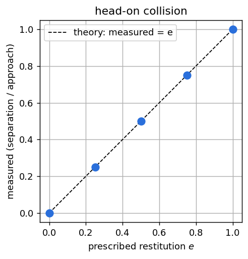
max |measured − e| = 0.00e+00; COM drift = 0.0e+002 — Bounce off a wall: height ratio is \(e^2\)
Drop a grain from height \(h\) onto a floor with restitution \(e\). Impact speed sets the rebound speed \(v_\text{out} = e\,v_\text{in}\), and height goes as \(v^2\), so the bounce height is \(e^2 h\). We run it against both an analytic plane and a signed-distance-field wall (a flat SDF floor, the same machinery a drum or hopper uses) — they must agree.
def drop(kind, e, h0=5.0, r=1.0):
    s = sim(1, restitution=e, gravity=(0, -9.8, 0))
    if kind == "plane":
        s.add_plane((0, 0, 0), (0, 1, 0))
    else:
        build_wall_sdf(lambda p: p[:, 1], ((-8, -3, -8), (8, 12, 8)), resolution=48).add_to(s, restitution=e)
    s.set_positions(np.array([[0, h0 + r, 0, 1]], np.float32))
    ys = []
    for _ in range(7000):
        s.step(0.002); ys.append(s.get_positions().reshape(-1, 3)[0, 1] - r)
    return np.array(ys)

fig, axes = plt.subplots(1, 2, figsize=(8.6, 3.6), sharey=True)
h0, e = 5.0, 0.7
for ax, kind in zip(axes, ["plane", "sdf"]):
    ys = drop(kind, e, h0)
    t = np.arange(len(ys)) * 0.002
    ax.plot(t, ys, color="#2a6fdb", lw=1.2)
    # successive-peak prediction e^(2k) h
    peak = max(ys[np.argmax(ys < 0.05):].max(), 0)  # first bounce apex
    for k in range(1, 5):
        ax.axhline(h0 * e**(2 * k), color="crimson", ls="--", lw=0.8)
    ax.set_xlabel("time"); ax.set_title(f"{kind} floor, e = {e}")
    record(f"bounce {kind}", peak / h0, e * e, 0.03)
axes[0].set_ylabel("height above floor")
plt.show()
print(f"first-bounce height / drop:  plane→{results['bounce plane'][0]:.3f}, "
      f"sdf→{results['bounce sdf'][0]:.3f}   (e² = {e*e:.3f})")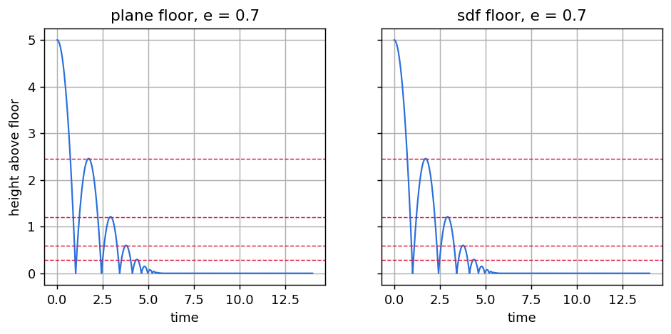
first-bounce height / drop: plane→0.492, sdf→0.492 (e² = 0.490)3 — Sliding grain spins up to rolling: \(v \to \tfrac{5}{7}v_0\)
A grain slid across a frictional floor with no initial spin is decelerated by friction while the same friction torque spins it up, until it rolls without slipping (\(v = \omega r\)). Angular-momentum bookkeeping for a solid sphere (\(I = \tfrac25 m r^2\)) gives the final speed exactly: \[ v_\text{roll} = \frac{v_0}{1 + I/(m r^2)} = \tfrac{5}{7}\,v_0. \]
v0, r = 3.0, 1.0
s = sim(1, restitution=0.0, friction=0.5, gravity=(0, -9.8, 0))
s.add_plane((0, 0, 0), (0, 1, 0))
s.set_positions(np.array([[0, r, 0, 1]], np.float32))
s.set_velocities(np.array([[v0, 0, 0]], np.float32))
V, SLIP = [], []
for _ in range(4000):
    s.step(0.002)
    v = s.get_velocities().reshape(-1, 3)[0, 0]
    w = s.get_angular_velocities().reshape(-1, 3)[0, 2]
    V.append(v); SLIP.append(v + w * r)          # contact-point (slip) velocity
V, SLIP = np.array(V), np.array(SLIP); t = np.arange(len(V)) * 0.002
record("rolling v/v0", V[-1] / v0, 5 / 7, 0.03)

fig, ax = plt.subplots(figsize=(5.2, 3.6))
ax.plot(t, V / v0, label="translational $v/v_0$", color="#2a6fdb")
ax.plot(t, SLIP / v0, label="slip $ (v+\\omega r)/v_0$", color="#e08a1e")
ax.axhline(5 / 7, color="crimson", ls="--", lw=1, label="theory $5/7$")
ax.axhline(0, color="0.6", lw=0.8)
ax.set_xlabel("time"); ax.set_ylabel("normalised"); ax.legend(); ax.set_title("sliding → rolling")
plt.show()
print(f"v_final/v0 = {V[-1]/v0:.3f}  (5/7 = {5/7:.3f});  residual slip = {SLIP[-1]:.2e}")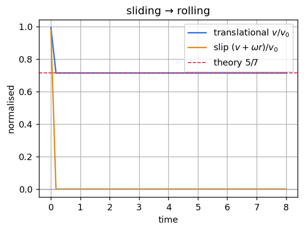
v_final/v0 = 0.714 (5/7 = 0.714); residual slip = 0.00e+004 — Column under gravity: a static, load-bearing stack
Six grains stacked in a column on a plate under gravity must settle into a static stack — the bottom grain carrying the weight of the five above it — without drifting, exploding, or interpenetrating. We check the assembly goes quiescent (velocities → 0) and the grains stay evenly stacked (centre-to-centre spacing = one diameter).
N, r = 6, 1.0
s = sim(N + 2, restitution=0.0, friction=0.3, gravity=(0, -9.8, 0))
s.add_plane((0, 0, 0), (0, 1, 0))
p = np.zeros((N, 4), np.float32)
p[:, 1] = [r + 2 * r * i for i in range(N)]   # touching column, centres a diameter apart
p[:, 3] = 1.0
s.set_positions(p)
VMAX, YS = [], []
for k in range(7000):
    s.step(0.002)
    VMAX.append(float(np.abs(s.get_velocities()).max()))
    if k % 50 == 0:
        YS.append(np.sort(s.get_positions().reshape(-1, 3)[:, 1]))
YS = np.array(YS)
gaps = np.diff(YS[-1])
record("column static |v|", VMAX[-1], 0.0, 0.15)
record("column spacing", float(gaps.mean()), 2 * r, 0.1)

fig, axes = plt.subplots(1, 2, figsize=(8.6, 3.6))
axes[0].plot(np.arange(len(VMAX)) * 0.002, VMAX, color="#2a6fdb")
axes[0].set_xlabel("time"); axes[0].set_ylabel("peak grain |v|"); axes[0].set_title("settling")
axes[0].set_yscale("log")
for i in range(N):
    axes[1].plot(np.arange(YS.shape[0]) * 50 * 0.002, YS[:, i], color="#2a6fdb", lw=1)
axes[1].set_xlabel("time"); axes[1].set_ylabel("grain height"); axes[1].set_title("stack (sorted)")
plt.show()
print(f"final peak |v| = {VMAX[-1]:.3f} (→0);  mean centre spacing = {gaps.mean():.3f} (diameter = {2*r})")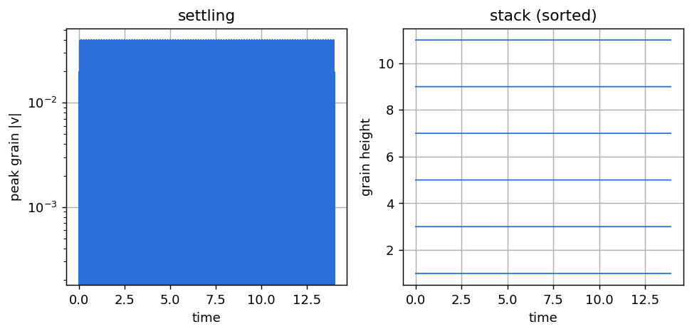
final peak |v| = 0.001 (→0); mean centre spacing = 2.000 (diameter = 2.0)5 — Spin meets friction: tangential deflection
Two grains collide head-on, each carrying spin. Friction acts on the relative surface velocity at the contact. If the grains co-rotate (both \(+\omega_z\)) their contact surfaces move in opposite directions → they slip → friction flings them apart transversely, symmetrically (\(v_y^A = -v_y^B\), by Newton’s third law). If they counter-rotate their surfaces move together → no slip → no deflection. The sign and symmetry of the kick validate the coupled friction/torque path.
def collide(spin):
    s = sim(2, restitution=0.2, friction=0.6)
    s.set_positions(np.array([[-3, 0, 0, 1], [3, 0, 0, 1]], np.float32))
    s.set_velocities(np.array([[2, 0, 0], [-2, 0, 0]], np.float32))
    s.set_angular_velocities(np.array([[0, 0, spin[0]], [0, 0, spin[1]]], np.float32))
    traj = []
    for _ in range(2600):
        s.step(0.002); traj.append(s.get_positions().reshape(-1, 3)[:, :2].copy())
    return np.array(traj), s.get_velocities().reshape(-1, 3)

fig, axes = plt.subplots(1, 2, figsize=(8.6, 3.8), sharex=True, sharey=True)
for ax, spin, ttl in [(axes[0], (10, 10), "co-rotating (both +ωz): slip → deflect"),
                      (axes[1], (10, -10), "counter-rotating (+ωz,−ωz): no slip")]:
    traj, v = collide(spin)
    for i, c in enumerate(["#2a6fdb", "#e08a1e"]):
        ax.plot(traj[:, i, 0], traj[:, i, 1], color=c, lw=1.5)
        ax.plot(traj[-1, i, 0], traj[-1, i, 1], "o", color=c, ms=6)
    ax.set_title(ttl, fontsize=9); ax.set_xlabel("x"); ax.set_aspect("equal")
    if spin == (10, 10):
        record("spin deflection symmetry", float(v[0, 1] + v[1, 1]), 0.0, 0.05)   # A = -B
        record("spin deflects", float(abs(v[0, 1])), 2.98, 1.0)                    # nonzero kick
    else:
        record("no-slip no deflection", float(abs(v[0, 1])), 0.0, 0.05)
axes[0].set_ylabel("y")
plt.show()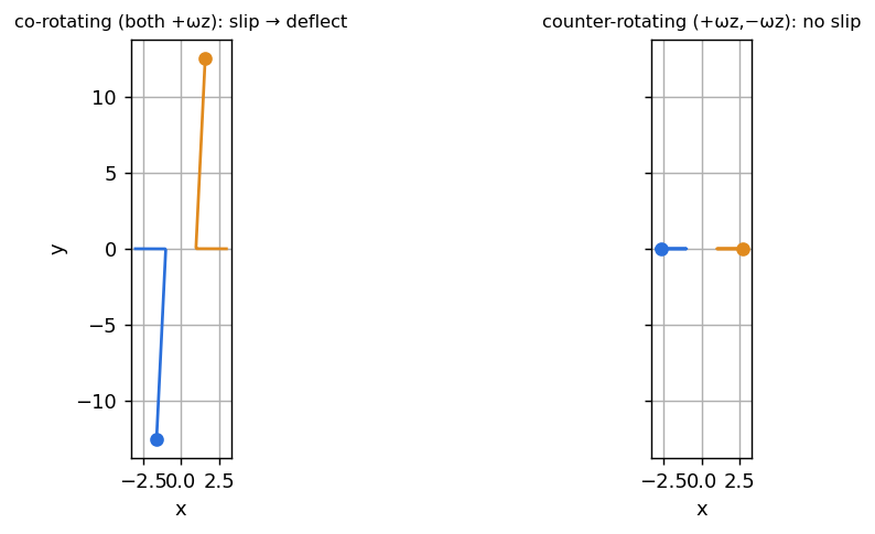
6 — A deep layered bed at rest: deep-stack statics
The hard case for any impulse-based contact solver is not one column of six grains but a deep bed: a thousand grains in forty touching layers, every contact loaded with the weight of everything above it. The static solution demands a complete force network — each contact carrying exactly its share — and any defect shows up as one of two failure signatures: grains interpenetrating at the bottom (the load “carried” by overlap), or a phantom velocity field (the bed looks static while the solver keeps re-lifting a falling state). Both are ruled out here with one number each: after two simulated seconds, the peak grain speed must be ~0, the minimum centre-to-centre spacing must still be one diameter, and the top layer must not have sunk.
The bed is a touching simple-cubic lattice (spacing exactly one diameter) on the plate, confined laterally by four snug walls so the frictionless-limit stack cannot buckle sideways — the load path runs straight down every column, the deepest-chain-per-grain configuration there is.
from scipy.spatial import cKDTree
r = 1.0
nx = nz = 5; nlay = 40
N = nx * nz * nlay
s = sim(N + 8, restitution=0.0, friction=0.3, gravity=(0, -9.8, 0))
s.add_plane((0, 0, 0), (0, 1, 0))                      # bottom plate
s.add_plane((-r, 0, 0), (1, 0, 0))                     # snug lateral confinement: boundary
s.add_plane((2 * r * (nx - 1) + r, 0, 0), (-1, 0, 0))  # grains exactly touch the walls
s.add_plane((0, 0, -r), (0, 0, 1))
s.add_plane((0, 0, 2 * r * (nz - 1) + r), (0, 0, -1))
ix, iy, iz = np.meshgrid(np.arange(nx), np.arange(nlay), np.arange(nz), indexing="ij")
p = np.zeros((N, 4), np.float32)
p[:, 0] = 2 * r * ix.ravel()
p[:, 1] = r + 2 * r * iy.ravel()                       # touching layers: centres a diameter apart
p[:, 2] = 2 * r * iz.ravel()
p[:, 3] = 1.0
p[:, [0, 2]] += np.random.default_rng(3).uniform(-1e-3, 1e-3, (N, 2)).astype(np.float32)
s.set_positions(p)
top0 = float(p[:, 1].max())

VMAX = []
for k in range(5000):
    s.step(0.002)
    if k % 10 == 0:
        VMAX.append(float(np.abs(s.get_velocities()).max()))
P = np.asarray(s.get_positions()).reshape(-1, 3)[:N]
nn = cKDTree(P).query(P, k=2)[0][:, 1]
record("bed peak |v|", VMAX[-1], 0.0, 0.15)
record("bed min spacing", float(nn.min()), 2 * r, 0.1)
record("bed top settle", float(P[:, 1].max()) - top0, 0.0, 0.3)

fig, axes = plt.subplots(1, 2, figsize=(8.6, 3.6))
axes[0].plot(np.arange(len(VMAX)) * 10 * 0.002, VMAX, color="#2a6fdb")
axes[0].set_xlabel("time"); axes[0].set_ylabel("peak grain |v|"); axes[0].set_yscale("log")
axes[0].set_title("the bed goes quiescent")
axes[1].plot(P[:, 1], nn, ".", ms=2, color="#2a6fdb", alpha=0.4)
axes[1].axhline(2 * r, color="crimson", ls="--", lw=1)
axes[1].set_xlabel("grain height"); axes[1].set_ylabel("nearest-neighbour distance")
axes[1].set_ylim(1.8, 2.2); axes[1].set_title("exact packing at every depth")
plt.show()
print(f"peak |v| = {VMAX[-1]:.4f} (→0);  min spacing = {nn.min():.4f} (diameter {2*r});  "
      f"top settle = {float(P[:,1].max()) - top0:+.4f}")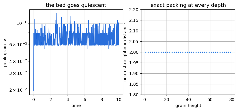
peak |v| = 0.0785 (→0); min spacing = 1.9998 (diameter 2.0); top settle = -0.0017
Note
This check is deliberately the deep version of check 4: pairwise, momentum-conserving contact impulses alone cannot hold a tall pile (the floor can only drain about one layer’s momentum per sweep), so the solver’s warm-started projected Gauss–Seidel + shock-propagation machinery is what is being exercised — and this is the check that trips if it regresses. It runs a thousand grains for 5,000 substeps: a couple of minutes on a laptop CPU, seconds on a GPU build.
Scorecard
check                           measured    expected   result
------------------------------------------------------------------
restitution e=0.0                 0.0000      0.0000   PASS ✅
restitution e=0.25                0.2500      0.2500   PASS ✅
restitution e=0.5                 0.5000      0.5000   PASS ✅
restitution e=0.75                0.7500      0.7500   PASS ✅
restitution e=1.0                 1.0000      1.0000   PASS ✅
bounce plane                      0.4918      0.4900   PASS ✅
bounce sdf                        0.4918      0.4900   PASS ✅
rolling v/v0                      0.7143      0.7143   PASS ✅
column static |v|                 0.0006      0.0000   PASS ✅
column spacing                    2.0000      2.0000   PASS ✅
spin deflection symmetry          0.0000      0.0000   PASS ✅
spin deflects                     2.9740      2.9800   PASS ✅
no-slip no deflection             0.0000      0.0000   PASS ✅
bed peak |v|                      0.0785      0.0000   PASS ✅
bed min spacing                   1.9998      2.0000   PASS ✅
bed top settle                   -0.0017      0.0000   PASS ✅
------------------------------------------------------------------
ALL CHECKS PASS ✅ (16/16)Adapt this yourself
- Add your own check. The pattern is always: a tiny setup with a closed-form answer, run, measure,
record(name, measured, expected, tol). Good candidates: oblique restitution, a two-grain Newton’s-cradle momentum transfer, terminal velocity under a dragset_external_forces, or the angle of repose of a heap. - Regression-guard a change. Run this page before and after touching the solver; the scorecard is a fast tripwire for physics regressions (this suite caught an energy-injection bug in the moving-wall contact solve).
- Non-spherical grains. Swap
set_sphere_shapefor an importedbuild_particleshape and re-check restitution and stacking — the collision model is the same point-shell-vs-SDF machinery.
Reproduce this
pip install -e '.[sim]'          # or: pip install peclet
PECLET_LOCAL_BUILD=/path/to/suite/dem/build_omp \
  quarto render sanity-checks/index.qmd --execute