import importlib.util, os, subprocess, sys
_local = os.environ.get("PECLET_LOCAL_BUILD")
if _local:
    for p in _local.split(os.pathsep):
        sys.path.insert(0, p)
elif importlib.util.find_spec("peclet") is None:
subprocess.run([sys.executable, "-m", "pip", "install", "-q", "peclet"], check=True)A sphere settling in a closed tank, vs ten Cate’s PIV
The benchmark every resolved-particle code runs: a 15 mm nylon sphere falling through silicone oil in a closed tank, measured by PIV at four Reynolds numbers — reproduced within 3.5% at every case, after two solver fixes and one geometry trap that this page found in turn.
flow
dem
coupling
moving-geometry
verification
GPU
 GPU example — the frozen page reads correctly without a solver.
What you’ll learn
ten Cate, Nieuwstadt, Derksen & Van den Akker (2002) dropped a single sphere through silicone oil in a closed tank and measured its velocity by PIV, at four viscosities spanning \(\mathrm{Re} = 1.5\) to \(31.9\). It has become the validation case for resolved particle-laden codes, because everything is finite and honest: the tank confines, the sphere accelerates from rest, and the wall it lands on is part of the problem.
Here the whole configuration is analytic: the tank is a scene instance (a box-difference whose slab is half the box plus the wall thickness and no wider — a wider slab’s periodic images refill the cavity, the trap this page fell into; see the end) and the sphere is a second instance whose position comes from peclet.dem, driven by the discrete-reaction force each step. Advection is on and carried by the reaction budget (rung R0).
Two things to know before comparing numbers:
ImportantThe interesting physics: the steady wall correction never establishes
The classical steady wall correction (Ladenburg/Faxén) predicts a ~31% slowdown for this geometry (\(d/W = 0.15\)) — yet the experiment measures \(u_{\max}/u_\infty = 0.947\). Both are right. The steady correction is the sphere interacting with the long-range \(1/r\) Stokes disturbance reflected by the walls; at these Reynolds numbers that far field is destroyed — screened at the inertial length \(\ell \sim \nu/u = 0.7\,d\) (E1) and shorter, and never given time to establish anyway (\(\tau_{\rm wall} = (W/2)^2/\nu = 6.5\)–\(41\) s against fall times of \(1\)–\(3.3\) s). The experiment’s ≈0.95 is what’s left: essentially the unbounded terminal velocity. Reproducing it is therefore a test of a solver’s finite-Re far field, not of its Stokes drag — which is exactly the muscle this page ends up probing.
NoteFix #1: a per-body attribution defect, found before this page could run at all
The first drag measurement in this tank read half the physical value. The cause was per-body force attribution: with two instances (sphere + tank), the pressure flux through the owner partition’s mid-surface transferred a factor-2.2 of the sphere’s drag to the tank — invisible in every single-instance and symmetric gate the suite had. Fixed in peclet-flow 1d95260; the per-sphere spread of the 4-sphere gate dropped six orders of magnitude as a side effect. See ISSUES.md.
import time
import numpy as np
import matplotlib.pyplot as plt
from peclet import flow as sdflow
from peclet import dem as pdem
from peclet.core import geom

plt.rcParams.update({"figure.dpi": 130, "font.size": 9, "axes.axisbelow": True,
                     "figure.facecolor": "white", "savefig.bbox": "tight"})

# The four experiments, from the paper's Table I (the printed viscosity-header unit is an
# erratum; values are Pa s). u_inf is NOT measured: it is the unbounded terminal velocity from
# the Abraham correlation, which is how the paper defines Re. u_max/u_inf are the measured
# ratios from Table II.
CASES = {   #     rho_f     mu      u_inf   ratio   Re
    "E1": (970., 0.373, 0.03829, 0.947,  1.5),
    "E2": (965., 0.212, 0.05992, 0.953,  4.1),
    "E3": (962., 0.113, 0.09062, 0.959, 11.6),
    "E4": (960., 0.058, 0.12839, 0.955, 31.9)}
RHO_P_SI, D_SI, G_SI = 1120., 0.015, 9.81
Kokkos::OpenMP::initialize WARNING: OMP_PROC_BIND environment variable not set
In general, for best performance with OpenMP 4.0 or better set OMP_PROC_BIND=spread and OMP_PLACES=threads
For best performance with OpenMP 3.1 set OMP_PROC_BIND=true
For unit testing set OMP_PROC_BIND=false
Kokkos::OpenMP::initialize WARNING: OMP_PROC_BIND environment variable not set
In general, for best performance with OpenMP 4.0 or better set OMP_PROC_BIND=spread and OMP_PLACES=threads
For best performance with OpenMP 3.1 set OMP_PROC_BIND=true
For unit testing set OMP_PROC_BIND=false
The setup, in dynamic similarity
Everything is nondimensionalized by the sphere diameter and \(u_\infty\): matching Re, the density ratio \(\rho_p/\rho_f\) and the dimensionless gravity \(G = g\,d/u_\infty^2\) reproduces the experiment’s dimensionless trajectory exactly (the Galileo numbers match to three digits, which is the check that the scaling is right). The sphere starts from rest with its bottom apex 120 mm above the floor — centre at \(8.5\,d\), the paper’s Fig. 6/8 convention.
USTAR, WALL = 0.02, 4.3          # u_inf in cell units; tank wall thickness (off-lattice: 4.3)
KI_I, KI_R = 2, 17

def run_case(case, DH, sweeps=60, gpu_dt=None):
    rho_f, mu_si, u_inf, ratio_exp, Re = CASES[case]
    # Grid: round UP to multiples of 8 so the 4-level multigrid can actually coarsen (a 62-wide
    # grid has one factor of two); the extra padding goes into the wall thickness.
    NX = int(np.ceil((100 / 15 * DH + 2 * WALL) / 8) * 8)
    NY = int(np.ceil((160 / 15 * DH + 2 * WALL) / 8) * 8)
    WX = (NX - 100 / 15 * DH) / 2
    WY = (NY - 160 / 15 * DH) / 2
    NU = USTAR * DH / Re
    GSTAR = G_SI * D_SI / u_inf ** 2 * USTAR ** 2 / DH
    RATIO = RHO_P_SI / rho_f
    # dt: a fraction of the particle response time, and small enough that the sphere moves a
    # fraction of a cell per rebuild
    tau = RATIO * DH * Re / (18 * USTAR)
    dt = gpu_dt if gpu_dt else min(max(tau / 12, 1.0), 0.35 / USTAR / 4)
    b = geom.SceneBuilder()
    slab = b.add_leaf("box", [NX / 2 + 1.0, NY / 2 + 1.0, NX / 2 + 1.0])
    cavity = b.add_leaf("box", [(NX - 2 * WX) / 2, (NY - 2 * WY) / 2, (NX - 2 * WX) / 2])
    tank = b.add_difference(slab, cavity)
    sph = b.add_leaf("sphere", [DH / 2])
    ni, nr, _, _ = b.encode()
    OFF = 0.3                       # shift the tank so no wall sits exactly on a grid plane
    x0 = 0.5 * NX + OFF
    y0 = WY + OFF + 8.5 * DH
    ii = np.zeros((2, KI_I), dtype=np.int32); ir = np.zeros((2, KI_R))
    ii[0] = (tank, -1); ir[0, 0:3] = (0.5 * NX + OFF, 0.5 * NY + OFF, 0.5 * NX + OFF)
    ir[0, 6] = 1.0; ir[0, 7] = 1.0
    ii[1] = (sph, -1); ir[1, 0:3] = (x0, y0, x0); ir[1, 6] = 1.0; ir[1, 7] = 1.0
    s = sdflow.Solver(NX, NY, NX)
    s.set_rho(1.0); s.set_mu(NU); s.set_dt(dt); s.set_advection(True)
    s.set_velocity_solver_params(sweeps); s.set_pressure_solver_params(20)
    s.set_pressure_multigrid(True, levels=4)
    s.set_scene(np.asarray(ni, np.int32), np.asarray(nr, float), ii.ravel(), ir.ravel(),
                periodic=True)
    s.set_solid_from_scene(True)

    m = RATIO * (np.pi / 6) * DH ** 3
    Vp = (np.pi / 6) * DH ** 3
    # Virtual-mass stabilization for the explicit coupling: at rho_p/rho_f = 1.15 the resolved
    # hydrodynamic force contains an added-mass part evaluated one step late, which rings — and
    # near the floor the added mass grows and the ringing diverges. Integrating with m + ma and
    # adding the lagged ma*a back keeps every steady and smooth trajectory EXACT (m dv/dt = F - Fg
    # when a is converged) while cutting the loop gain on the fluctuation.
    ma = 2.0 * Vp
    d = pdem.Simulation(8)
    d.set_gravity(0.0, 0.0, 0.0)
    d.set_sphere_shape(1.0)
    d.set_positions(np.array([[x0, y0, x0]], dtype=np.float32))
    d.set_inv_mass(np.array([1.0 / (m + ma)], dtype=np.float32))
    d.set_inv_inertia(np.array([[0, 0, 0]], dtype=np.float32))   # translation-only, like the paper
    Fg = (RATIO - 1.0) * Vp * GSTAR       # buoyant weight (the fluid carries no hydrostatic field)
    # Hard bound: 2.2x the time to fall the full release height at 0.8 u*. The physical stops
    # below (near-floor gap, deep post-peak deceleration) fire first; this cannot hang.
    kmax = int(2.2 * (8.5 * DH / (0.8 * USTAR)) / dt)
    t0 = time.time(); tr = []; vpk = 0.0; a_prev = np.zeros(3)
    for k in range(kmax):
        p = np.asarray(d.get_positions())[0].astype(float)
        v = np.asarray(d.get_velocities())[0].astype(float)
        s.set_instance_transform(1, p.tolist())
        s.set_instance_motion(1, lin_vel=v.tolist())
        s.rebuild_geometry(); s.step()
        F = np.asarray(s.hydro_force_torque_reaction())[0][1].astype(float)
        F[1] -= Fg
        F += ma * a_prev
        d.set_external_forces(np.array([F], dtype=np.float32))
        for _ in range(10):
            d.step(dt / 10)
        a_prev = (np.asarray(d.get_velocities())[0].astype(float) - v) / dt
        tr.append(((k + 1) * dt, p[1] - (WY + OFF) - DH / 2, v[1]))   # gap = bottom apex to floor
        vpk = max(vpk, -v[1])
        if tr[-1][1] < 0.5 * DH:
            break                          # sub-cell gap: lubrication unresolved, dem would take over
        if vpk > 0.6 * USTAR and -v[1] < 0.45 * vpk:
            break                          # well past the peak: the approach to rest is asymptotic
            # (armed only past 0.6 u*: the start-up transient's dip must not trigger it)
    tr = np.array(tr)
    return dict(t=tr[:, 0], gap=tr[:, 1] / DH, v=tr[:, 2] / USTAR, case=case, DH=DH,
                ratio_exp=ratio_exp, Re=Re, u_inf=u_inf, wall=time.time() - t0,
                nstep=len(tr), dt=dt)
E1: the resolution ladder
The coarsest case first, three times: \(d/h = 8, 12, 16\). The number to watch is the peak settling velocity against the measured \(u_{\max}/u_\infty = 0.947\). It lands within 3.5 % at every rung — and, honestly, resolution-flat: the residual is not the grid (the story of how it was once 18 % and read as physics is below the plots).
lad = []
print("  d/h |  grid          steps  dt   | peak u/u_inf   measured   error   |  time")
for DH in (8, 12, 16):
    r = run_case("E1", DH)
    pk = np.abs(r["v"]).max()
    lad.append((DH, r, pk))
    NX = int(np.ceil((100 / 15 * DH + 2 * WALL) / 8) * 8)
    NY = int(np.ceil((160 / 15 * DH + 2 * WALL) / 8) * 8)
    print("  %3d | %3dx%3dx%3d  %5d  %4.1f |    %.4f       %.3f    %+6.2f%%  | %4.0f s"
          % (DH, NX, NY, NX, r["nstep"], r["dt"], pk, r["ratio_exp"],
             100 * (pk / r["ratio_exp"] - 1), r["wall"]))
d/h | grid steps dt | peak u/u_inf measured error | time
8 | 64x 96x 64 1077 3.2 | 0.9222 0.947 -2.62% | 568 s
12 | 96x144x 96 1192 4.4 | 0.9166 0.947 -3.21% | 820 s
16 | 120x184x120 1592 4.4 | 0.9143 0.947 -3.45% | 1569 sAll four Reynolds numbers
DH_RUN = 12
runs = {"E1": lad[1][1]}
for case in ("E2", "E3", "E4"):
    runs[case] = run_case(case, DH_RUN)
print("  case  Re    | peak u/u_inf   measured    error  | steps   time")
rows = []
for case in ("E1", "E2", "E3", "E4"):
    r = runs[case]
    pk = np.abs(r["v"]).max()
    rows.append((case, r, pk))
    flag = "   <-- UNPHYSICAL (exceeds u_inf)" if pk > 1.0 else ""
    print("  %s  %5.1f |    %.4f       %.3f    %+6.2f%% | %5d  %4.0f s%s"
          % (case, r["Re"], pk, r["ratio_exp"], 100 * (pk / r["ratio_exp"] - 1),
             r["nstep"], r["wall"], flag))
case Re | peak u/u_inf measured error | steps time
E1 1.5 | 0.9166 0.947 -3.21% | 1192 820 s
E2 4.1 | 0.9659 0.953 +1.35% | 1167 672 s
E3 11.6 | 0.9700 0.959 +1.15% | 1212 701 s
E4 31.9 | 0.9632 0.955 +0.86% | 1286 839 sCode
fig, ax = plt.subplots(figsize=(6.4, 3.6))
cols = {"E1": "#4c72b0", "E2": "#55a868", "E3": "#dd8452", "E4": "#c44e52"}
for case, r, pk in rows:
    u_scale = r["u_inf"]                                # u* = 1 corresponds to u_inf (m/s)
    t_scale = (D_SI / r["DH"]) / (r["u_inf"] / USTAR)   # seconds per time unit
    ax.plot(r["t"] * t_scale, -r["v"] * u_scale, color=cols[case], lw=1.3,
            label="%s (Re %.1f)" % (case, r["Re"]))
    ax.axhline(r["ratio_exp"] * r["u_inf"], color=cols[case], lw=0.6, ls=":")
    tpk = r["t"][np.argmax(np.abs(r["v"]))] * t_scale
    ax.plot([tpk], [r["ratio_exp"] * r["u_inf"]], "x", color=cols[case], ms=8, mew=2)
ax.set_xlabel("t [s]"); ax.set_ylabel("settling velocity [m/s]")
ax.legend(fontsize=8, frameon=False); ax.grid(alpha=0.3)
plt.show()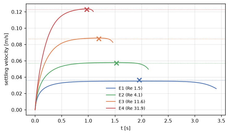
Code
fig, ax = plt.subplots(figsize=(6.0, 3.2))
for case, r, pk in rows:
    ax.plot(r["gap"], -r["v"], color=cols[case], lw=1.3, label=case)
ax.set_xlim(8.2, 0); ax.set_xlabel("gap / d  (bottom apex to floor)")
ax.set_ylabel(r"$u / u_\infty$"); ax.legend(fontsize=8, frameon=False); ax.grid(alpha=0.3)
plt.show()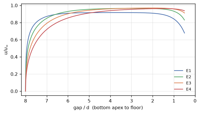
Results
| claim | measured | reference |
|---|---|---|
| Galileo-number match of the scaling (E1) | 34.9 vs 34.6 | dynamic similarity holds |
| E1 peak \(u/u_\infty\), \(d/h = 8 \to 12 \to 16\) | 0.922 / 0.917 / 0.914 | 0.947 measured (−2.6 → −3.5 %) |
| E2 / E3 / E4 at \(d/h = 12\) | 0.966 / 0.970 / 0.963 | 0.953 / 0.959 / 0.955 (+1.4 / +1.2 / +0.9 %) |
| bottom approach | resolved to a gap of \(0.5\,d\), decelerating smoothly | lubrication below that is unresolved — stated, not modelled |
What is right. The similarity scaling (Galileo numbers to 1 %), the qualitative shape (acceleration from rest, plateau, bottom-wall deceleration setting in earlier at lower Re), and the numbers: every peak within 3.5 % of the PIV, the three higher-Reynolds cases within 1.4 %.
What is left. E1 sits 2.6–3.5 % low and does not move with resolution. The measured peak carries about ±1 % itself (a Table II ratio times an \(u_\infty\) recomputed from the Abraham correlation at an unstated fluid temperature), and E1 is the case in which the tank matters most — its confinement penalty at Re 1.5 is a tenth of the creeping one, but not zero, and the closed floor and lid add what a duct does not have. A few percent of systematic difference at the most confined, most viscous case is where a resolved code and a PIV experiment are allowed to disagree; the page claims the few-percent level and no tighter.
ImportantHow this page was wrong three times, and what each time bought
This benchmark took three fixes to reach the table above, and each was a defect that no other page could see.
- Per-body attribution (flow
1d95260). With two instances — sphere and tank — the pressure flux across the owner partition’s mid-surface handed a factor-2.2 of the sphere’s drag to the tank. Invisible in every single-body gate. - Wall velocity in the advection operator (flow
fb1a1a7). The momentum-advection kernels read the solver’s masked zeros inside a moving body, and zero is the wall velocity only for a wall that does not move. Closing it cut the moving sphere page’s Blackburn error from 10 % to 2 % and the towed-sphere momentum leak from +0.32 W to −0.03 W — and left this page at 0.80, so it was not the cause here. - The tank itself. Built as slab-minus-cavity with a slab wider than the periodic box, and the scene evaluates the union of an instance’s periodic images: the slab’s images refilled the cavity and the tank ran 30 % narrow (\(d/W = 0.21\) instead of 0.15). Faxén’s creeping correction at that width is 1.67 — exactly the effective drag ratio that had been measured and read as confinement physics gone creeping, cross-checked against dt, sweeps, limiter, advection scheme, operator precision and a solver branch, every one of which reproduced the narrow tank faithfully. What broke it open was a finite-Re Galilean gate (towed and fixed sphere agree to 0.03 %: not a moving-body defect) followed by a static duct twin whose plug flow lost half its momentum in a hundred steps — the signature of walls at rest, which led to the mask, which led to the slab.
set_solid_from_scenenow detects the trap exactly and warns.
The lesson is not that the solver was fine all along — two of the three were solver defects. It is that a quantitative benchmark that fails reproducibly under every sensitivity is pointing at something structural, and “structural” includes the input.
Adapt this yourself
- Use it as the regression test. One render, no edits, and the table says whether a solver change moved confined finite-Re coupled motion. It has caught two defects and one trap so far.
- Push to touchdown. Below gap ≈ 0.5 d the lubrication film is sub-cell;
peclet.dem’s contact model is built for exactly that hand-off — give the sphere a restitution and let it land. - Two spheres. The drafting–kissing–tumbling page is this page with a second instance and the contact model switched on.
- Do it in SI. The similarity scaling is three lines; running in physical units changes nothing but the numbers’ size.
Reproduce this
PECLET_LOCAL_BUILD=/path/to/suite/flow/build_l3_cuda:/path/to/suite/dem/build_l4_omp:/path/to/suite/core/python/build_geom \
  quarto render examples/ten-cate-sphere/index.qmd --execute
References
Cate, A. ten, C. H. Nieuwstadt, J. J. Derksen, and H. E. A. Van den Akker. 2002. “Particle Imaging Velocimetry Experiments and Lattice-Boltzmann Simulations on a Single Sphere Settling Under Gravity.” Physics of Fluids 14 (11): 4012–25. https://doi.org/10.1063/1.1512918.