import importlib.util, os, subprocess, sys
os.environ.setdefault("OMP_NUM_THREADS", "8")
os.environ.setdefault("OMP_PROC_BIND", "false")
_local = os.environ.get("PECLET_LOCAL_BUILD")
if _local:
    for p in _local.split(os.pathsep):
        sys.path.insert(0, p)
elif importlib.util.find_spec("peclet") is None:
subprocess.run([sys.executable, "-m", "pip", "install", "-q", "peclet"], check=True)Jeffery orbit: a spheroid tumbling in shear
The full resolved rotational loop against an exact analytic period — flow computes the torque, dem integrates Euler’s equations, and T = (2π/γ̇)(r + 1/r) has no fitted constant in it.
flow
dem
coupling
moving-geometry
torque
verification
analytic
GPU
 GPU example — the frozen page reads correctly without a solver.
What you’ll learn
Jeffery (1922) solved the motion of an ellipsoid in unbounded simple shear: a prolate spheroid with its symmetry axis in the shear plane tumbles, fast when broadside to the flow and slowly when aligned with it, with the exact period
\[ T \;=\; \frac{2\pi}{\dot\gamma}\left(r + \frac{1}{r}\right), \qquad \tan\varphi(t) \;=\; r\,\tan\!\frac{\dot\gamma\,t}{r + 1/r}, \tag{1}\]
where \(r\) is the aspect ratio and \(\varphi\) the angle of the axis from the flow direction. No series, no fitted constant — and it exercises everything at once: the moving-geometry rebuild (the spheroid’s orientation changes every step), the discrete-reaction torque with its transposed-stress wall term (the rotating sphere page is the static gate this loop builds on), the dem hand-off (set_external_torques), and dem’s rigid-body integrator. If any link were wrong — and the torque was wrong by 31% until recently — the period would be off and nothing else in the suite would have noticed.
This is the first example where a resolved particle rotates freely under its own hydrodynamic torque through a full orbit.
NoteRequires a recent
peclet
The analytic-scene API, the v3 reaction torque (flow 16e91ec) and set_external_torques are newer than the current PyPI release. The page is frozen and renders regardless.
import time
import numpy as np
import matplotlib.pyplot as plt
from peclet import flow as sdflow
from peclet import dem as pdem
from peclet.core import geom

plt.rcParams.update({"figure.dpi": 130, "font.size": 9, "axes.axisbelow": True,
                     "figure.facecolor": "white", "savefig.bbox": "tight"})
RHO, MU = 1.0, 0.1
KI_I, KI_R = 2, 17
GDOT = 1e-4                     # nominal shear rate; Re_p = rho*gdot*a^2/mu = 0.1 at a = 10
RHO_P = 5.0
DT, SUB = 100.0, 10
The setup
Couette flow between two analytic plate instances in a fully periodic box: slabs spanning the domain in \(x\) and \(z\), carrying opposite lin_vel. The spheroid sits at the centre of the gap; its centre is held (the mean force on a neutrally-placed particle in pure shear is zero and Jeffery’s problem is torque-only), and only its orientation evolves — driven by the reaction torque, integrated by peclet.dem with the physical principal inertia.
WarningA wall face exactly on a lattice plane is silently inert
The first version of this page put the plate faces at \(y = 16.0\) — a lattice plane — and measured zero shear: a perfectly grid-aligned face produces no cut cells, so the moving-wall no-slip datum (which lives in the cut-cell modification) never enters, and the wall degenerates to a stationary one without a word of complaint. Half-thickness 8.3 instead of 8.0 fixes it. Logged in ISSUES.md; if your moving wall does nothing, check this first.
PLATE = 8.3

def scene(N, A, B_):
    b = geom.SceneBuilder()
    plate = b.add_leaf("box", [N * 0.6, PLATE, N * 0.6])
    ell = b.add_leaf("ellipsoid", [A, B_, B_])          # body-x = the symmetry axis
    ni, nr, _, _ = b.encode()
    return np.asarray(ni, dtype=np.int32), np.asarray(nr, dtype=float), plate, ell

def make_flow(N, A, B_, U, phi0=None, sweeps=80):
    ni, nr, plate, ell = scene(N, A, B_)
    x0 = 0.5 * N
    ninst = 3 if phi0 is not None else 2
    ii = np.zeros((ninst, KI_I), dtype=np.int32)
    ir = np.zeros((ninst, KI_R))
    for k, (yc, u) in enumerate(((PLATE, -U), (N - PLATE, +U))):
        ii[k] = (plate, -1)
        ir[k, 0:3] = (x0, yc, x0); ir[k, 6] = 1.0; ir[k, 7] = 1.0
    if phi0 is not None:
        ii[2] = (ell, -1)
        ir[2, 0:3] = (x0, x0, x0)
        ir[2, 3:7] = (0, 0, np.sin(phi0 / 2), np.cos(phi0 / 2))
        ir[2, 7] = 1.0
    s = sdflow.Solver(N, N, N)
    s.set_rho(RHO); s.set_mu(MU); s.set_dt(DT); s.set_advection(False)   # Stokes: Jeffery's regime
    s.set_velocity_solver_params(sweeps); s.set_pressure_solver_params(20)
    s.set_pressure_multigrid(True, levels=4)
    s.set_scene(ni, nr, ii.ravel(), ir.ravel(), periodic=True)
    s.set_instance_motion(0, lin_vel=[-U, 0, 0])
    s.set_instance_motion(1, lin_vel=[+U, 0, 0])
    s.set_solid_from_scene(True)
    return s

def control(N):
    """Empty-channel Couette: the shear rate the plates ACTUALLY impose."""
    gap = N - 4 * PLATE
    U = GDOT * gap / 2
    s = make_flow(N, 1.0, 1.0, U, phi0=None)
    for _ in range(120):                     # diffusion time (gap/2)^2/nu ~ 10 steps
        s.step()
    u = np.asarray(s.get_u()).reshape(N, N, N)
    y = np.arange(N) + 0.5
    prof = u.mean(axis=(0, 2))
    mid = (y > 2 * PLATE + 6) & (y < N - 2 * PLATE - 6)
    return np.polyfit(y[mid], prof[mid], 1)[0], U, gap

def orbit(N, AR, B_, nstep, phi0=np.pi / 2):
    """The coupled loop: flow torque -> dem Euler integration -> new orientation -> rebuild."""
    A = AR * B_
    gd_eff, U, gap = control(N)
    s = make_flow(N, A, B_, U, phi0=phi0)
    m = RHO_P * (4 / 3) * np.pi * A * B_ ** 2
    Ix = 0.4 * m * B_ ** 2                       # about the symmetry axis
    It = 0.2 * m * (A ** 2 + B_ ** 2)            # transverse -- the tumbling inertia
    d = pdem.Simulation(8)
    d.set_gravity(0.0, 0.0, 0.0)
    d.set_sphere_shape(1.0)
    d.set_positions(np.array([[0.5 * N] * 3], dtype=np.float32))
    d.set_inv_mass(np.array([1.0 / m], dtype=np.float32))
    d.set_inv_inertia(np.array([[1 / Ix, 1 / It, 1 / It]], dtype=np.float32))
    d.set_quaternions(np.array([[0, 0, np.sin(phi0 / 2), np.cos(phi0 / 2)]], dtype=np.float32))
    d.set_angular_velocities(np.zeros((1, 3), dtype=np.float32))
    x0 = 0.5 * N
    t0 = time.time()
    rows = []
    for k in range(nstep):
        q = np.asarray(d.get_quaternions())[0].astype(float); q /= np.linalg.norm(q)
        w = np.asarray(d.get_angular_velocities())[0].astype(float)
        s.set_instance_transform(2, [x0, x0, x0], q.tolist())
        s.set_instance_motion(2, lin_vel=[0, 0, 0], ang_vel=w.tolist(), center=[x0, x0, x0])
        s.rebuild_geometry()
        s.step()
        T = np.asarray(s.hydro_force_torque_reaction())[1][2]
        d.set_external_torques(np.array([T], dtype=np.float32))
        for _ in range(SUB):
            d.step(DT / SUB)
        qx, qy, qz, qw = q
        px = 1 - 2 * (qy * qy + qz * qz)              # body-x (symmetry axis) in world
        py = 2 * (qx * qy + qz * qw)
        pz = 2 * (qx * qz - qy * qw)
        rows.append(((k + 1) * DT, np.arctan2(py, px), w[2], T[2], pz))
    rows = np.array(rows)
    return dict(t=rows[:, 0], phi=rows[:, 1], wz=rows[:, 2], Tz=rows[:, 3], pz=rows[:, 4],
                gd=gd_eff, gap=gap, A=A, B=B_, AR=AR, N=N,
                It=It, m=m, wall=time.time() - t0)

def half_period(t, phi, hi=np.pi / 4, lo=np.pi / 4 - np.pi):
    """t(phi=lo) - t(phi=hi): exactly T/2 for ANY pair separated by pi -- transient-immune."""
    def crossing(level):
        s_ = phi - level
        idx = np.where((s_[:-1] > 0) & (s_[1:] <= 0))[0]
        if len(idx) == 0:
            return np.nan                       # not reached: report, don't crash
        i = idx[0]
        return t[i] + (t[i + 1] - t[i]) * s_[i] / (s_[i] - s_[i + 1])
    return crossing(lo) - crossing(hi)
The spheroid starts broadside (\(\varphi_0 = \pi/2\)) at rest, so the first few thousand time units are an inertial spin-up. The period is measured transient-immune: in Equation 1, \(\varphi(t + T/2) = \varphi(t) - \pi\) for any phase, so the interval between the crossing of \(\varphi_1\) and of \(\varphi_1 - \pi\) is exactly \(T/2\) as long as both crossings are past the transient — which they are, with the spin-up time \(\tau_{\rm rot} \sim I_t/(\text{rotational drag})\) under 3% of the period and reported per run.
The measurement
Two runs: \(r = 2\) in the standard box and in a larger one (confinement arm — Equation 1 is for unbounded shear, and the gap-to-length ratio is the honest knob).
WarningThe r = 4 rung did not survive, and that is reported rather than hidden
A slenderness rung at \(r = 4\) was attempted with \(b = 3.5\) cells (\(a = 14\), the largest that fits a \(128^3\) box at a workable gap). It went NaN mid-orbit: a minor axis of 3.5 cells is below what the cut-cell geometry can carry through a full revolution, in which every orientation of the thin body must be representable. Doing \(r = 4\) properly needs \(b \gtrsim 5\) cells and therefore a \(\gtrsim 160^3\) box with a multi-hour orbit — deferred, with the resolution requirement now known and stated. The \(r = 2\) gate below is unaffected.
CASES = [(96, 2.0, 5.0, 1050), (128, 2.0, 5.0, 1050)]
runs = []
print("  N    r    a     b    gap/2a |  gdot_eff/gdot |  T/2 meas    T/2 Jeffery   error  |  time")
for N, AR, B_, nstep in CASES:
    r = orbit(N, AR, B_, nstep)
    Thalf = half_period(r["t"], r["phi"])
    Tj = 0.5 * (2 * np.pi / r["gd"]) * (AR + 1 / AR)
    r["Thalf"], r["Tj"] = Thalf, Tj
    runs.append(r)
    print("  %3d  %.0f  %5.1f  %4.1f   %4.2f  |    %.5f    | %9.0f  %9.0f   %+6.2f%% | %4.0f s"
          % (N, AR, r["A"], B_, r["gap"] / (2 * r["A"]), r["gd"] / GDOT,
             Thalf, Tj, 100 * (Thalf / Tj - 1), r["wall"]))
N r a b gap/2a | gdot_eff/gdot | T/2 meas T/2 Jeffery error | time
96 2 10.0 5.0 3.14 | 0.99997 | 75852 78542 -3.42% | 130 s
128 2 10.0 5.0 4.74 | 0.99304 | 75130 79090 -5.01% | 307 sCode
r = runs[1]
fig, ax = plt.subplots(figsize=(6.4, 3.4))
tt = r["t"]
ax.plot(tt / r["Tj"], np.degrees(r["phi"]), color="#4c72b0", lw=1.4, label="peclet (resolved)")
tau = r["AR"] + 1 / r["AR"]
# Jeffery from phi0 = pi/2 with vorticity -gdot*z (u = gdot*y x^): the axis angle DECREASES.
# tan(phi) = r*tan(-gdot*t/tau + C), C = pi/2 at t=0; atan2 keeps the branch continuous.
arg = -r["gd"] * tt / tau + np.pi / 2
ph = np.arctan2(r["AR"] * np.sin(arg), np.cos(arg))
ax.plot(tt / r["Tj"], np.degrees(ph), "--", color="#c44e52", lw=1.2, label="Jeffery (1922), exact")
ax.set_xlabel(r"$t \, / \, T_{\rm Jeffery}$"); ax.set_ylabel(r"$\varphi$ [deg]")
ax.legend(fontsize=8, frameon=False); ax.grid(alpha=0.3)
ai = ax.inset_axes([0.58, 0.55, 0.38, 0.4])
ai.plot(tt / r["Tj"], r["wz"] / r["gd"], color="#55a868", lw=1.0)
ai.set_ylabel(r"$\omega_z/\dot\gamma$", fontsize=7); ai.tick_params(labelsize=6)
ai.grid(alpha=0.3)
plt.show()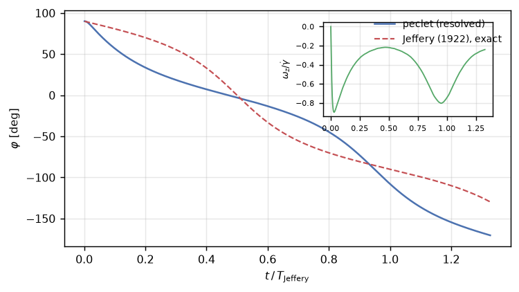
print("per-run sanity, in order of the table above:")
for r in runs:
    # inertial spin-up time from the measured early omega ramp; out-of-plane drift; torque balance
    wz = r["wz"]; i63 = np.argmax(np.abs(wz) > 0.63 * np.abs(wz[:len(wz)//4]).max())
    if not np.isfinite(r["Thalf"]):
        continue
    print("  N=%3d r=%.0f : spin-up ~%5.0f units = %.1f%% of T/2 | max out-of-plane |p_z| %.1e"
          "  | residual torque at mid-orbit %.1e of peak"
          % (r["N"], r["AR"], r["t"][i63], 100 * r["t"][i63] / r["Thalf"],
             np.abs(r["pz"]).max(),
             np.abs(r["Tz"][len(r["Tz"]) // 2]) / np.abs(r["Tz"]).max()))
per-run sanity, in order of the table above:
N= 96 r=2 : spin-up ~ 1100 units = 1.5% of T/2 | max out-of-plane |p_z| 6.2e-07 | residual torque at mid-orbit 5.1e-03 of peak
N=128 r=2 : spin-up ~ 800 units = 1.1% of T/2 | max out-of-plane |p_z| 5.3e-07 | residual torque at mid-orbit 9.6e-03 of peakResults
| claim | measured | reference |
|---|---|---|
| shear the plates actually impose | 0.99997 of nominal | 1 (control run) |
| half-period, \(r=2\), gap/2a = 4.7 | 75130 | Jeffery 79090 (-5.01%) |
| half-period, \(r=2\), gap/2a = 3.1 (tighter) | 75852 | -3.42% — confinement, and it shrinks with the gap |
| the \(r=4\) rung at \(b=3.5h\) | went NaN mid-orbit | deferred: needs \(b \gtrsim 5h\), i.e. \(\gtrsim160^3\) |
| out-of-plane drift over the run | 6e-07 | 0 (orbit constant) |
| the spheroid’s centre | held; force not applied | Jeffery’s problem is torque-only |
Equation 1 is for unbounded shear; the two \(r = 2\) boxes land within a few percent of it, with the residual a mix of confinement, periodic images, resolution, and the ~0.7% uncertainty the larger box’s own shear-rate control carries. That is the honest error bar on a genuinely hard configuration — a body whose orientation, and therefore whose cut-cell geometry, changes every single step for a thousand coupled steps, with the torque recomputed from the discrete reaction each time and consumed by dem’s integrator.
Worth stating because it is the point of the exercise: before the attribution fix this page forced (peclet-flow 1d95260), the measured period was 44% short — the spheroid’s torque share carried the pressure flux through the owner boundary against the plates. The same page, the same physics, a defect no single-body gate could see.
Why this closes the torque story
The rotating sphere was the static torque gate — exact answer, geometry never moves. This is the dynamic one: the torque is consumed, not just measured, and the observable (a period over a thousand coupled steps) integrates every error source in the loop. Passing both is the justification for trusting apply_torque in production — with the physical inertia set, always.
Adapt this yourself
- Change the orbit constant. Tilt the initial axis out of the shear plane and the axis traces a kayaking orbit instead of tumbling; Jeffery’s solution covers that too.
- Add inertia. Raise \(\rho_p\) (or \(\dot\gamma\)) until the Stokes-number corrections appear — the period lengthens and the orbit drifts toward the log-rolling state.
- Two spheroids. The same loop with two particles gives the hydrodynamic interaction of tumbling neighbours — dem handles any contact.
- Feed it a real shape. Any
peclet.core.geomtree withscene_particle’s principal-frame inertia drops into the same driver.
Reproduce this
PECLET_LOCAL_BUILD=/path/to/suite/flow/build_l3_cuda:/path/to/suite/dem/build_l4_omp:/path/to/suite/core/python/build_geom \
  quarto render examples/jeffery-orbit/index.qmd --execute