# Makes this notebook run out-of-the-box on Colab/Binder. A real user just needs the
# published package; this installs it on first run. Authors can instead point at a
# local source build of the suite with the PECLET_LOCAL_BUILD env var.
import importlib.util, os, subprocess, sys
_local = os.environ.get("PECLET_LOCAL_BUILD")
if _local:
    sys.path.insert(0, _local)                                  # local source build
elif importlib.util.find_spec("peclet") is None:
subprocess.run([sys.executable, "-m", "pip", "install", "-q", "peclet"], check=True)Rising bubble: the Hysing benchmark, both cases
A buoyant bubble in a viscous liquid at density ratios 10 and 1000 — rise velocity and centroid against the published reference, and the momentum-consistent transport that buys a factor five.
flow
vof
two-phase
surface-tension
buoyancy
benchmark
gpu
 Three runs of a few thousand steps each — comfortable on a GPU build, slow but possible on a Colab CPU runtime at half the resolution.
What you’ll learn
How to run a real two-phase problem with peclet’s geometric VoF: buoyancy as a closure of the colour field, a variable density and viscosity, balanced-force surface tension, and the adaptive time step that two explicit stability limits jointly dictate. The yardstick is the benchmark everybody uses — Hysing et al. (Hysing et al. 2009), who ran the same bubble with three independent codes and published the numbers they agree on.
Two results worth the page on their own:
- Case 1 (density ratio 10, Eötvös 10) reproduces the reference centroid at \(t=3\) to 0.02 % and the peak rise velocity to +3.3 %.
- Turning momentum-consistent transport off — advecting \(\rho\mathbf{u}\) with a different flux than \(C\), which is what most simple VoF implementations do — multiplies the case-1 peak-velocity error by five (and the centroid error by nearly three orders of magnitude), at density ratio 10 — an order of magnitude below where the literature says consistency starts to matter (Rudman 1998; Arrufat et al. 2021).
You will also see, in the same run, the two explicit limits trade places: the capillary time step binds throughout case 1, and the transport CFL takes over in case 2.
The problem
A circular gas bubble of radius \(r=0.25\) starts at rest, centred at \((0.5, 0.5)\) in a \(1\times2\) box of heavier liquid, and rises under gravity. The governing equations are the incompressible Navier–Stokes equations with a single, variable density and viscosity field and a singular interfacial force:
\[ \partial_t(\rho\mathbf{u}) + \nabla\!\cdot\!(\rho\mathbf{u}\mathbf{u}) = -\nabla p + \nabla\!\cdot\!\big[\mu(\nabla\mathbf{u}+\nabla\mathbf{u}^{\mathsf T})\big] + \rho\mathbf{g} + \sigma\kappa\,\mathbf{n}\,\delta_S , \qquad \nabla\!\cdot\!\mathbf{u}=0 \tag{1}\]
\[ \partial_t C + \nabla\!\cdot\!(C\,\mathbf{u}) = 0, \qquad \rho = \rho_2 + (\rho_1-\rho_2)\,C, \qquad \mu = \mu_2 + (\mu_1-\mu_2)\,C \tag{2}\]
with \(C\) the liquid volume fraction (so the bubble is \(C=0\)). The benchmark fixes two dimensionless groups, built on the bubble diameter \(d=2r\) and the gravitational velocity scale \(U_g=\sqrt{g\,d}\):
\[ \mathrm{Re} = \frac{\rho_1 U_g d}{\mu_1}, \qquad \mathrm{Eo} = \frac{\rho_1 U_g^2 d}{\sigma} = \frac{\rho_1 g d^2}{\sigma} \tag{3}\]
Case 1 (\(\rho_1/\rho_2 = 10\), \(\mu_1/\mu_2 = 10\), \(\mathrm{Re}=35\), \(\mathrm{Eo}=10\)) stays an ellipse: surface tension is strong enough to hold the shape, all three reference codes agree to three digits, and it is the case a solver has no excuse for. Case 2 (\(\rho_1/\rho_2 = 1000\), \(\mu_1/\mu_2 = 100\), \(\mathrm{Eo}=125\)) is the hard one: the bubble becomes a skirted cap, thin filaments form at the trailing edge, and the reference codes themselves disagree — Hysing et al. report \(y_c(3) = 1.1249\), \(1.1376\) and \(1.1512\) and state the case is not grid-converged.
The two quantities we report are the ones computable from the colour field alone:
\[ y_c(t) = \frac{\int_{\Omega_b} y \,\mathrm{d}\Omega}{\int_{\Omega_b} \mathrm{d}\Omega}, \qquad V_c(t) = \frac{\int_{\Omega_b} u_y \,\mathrm{d}\Omega}{\int_{\Omega_b} \mathrm{d}\Omega}, \qquad \Omega_b = \{1-C\} \tag{4}\]
NoteTwo honest caveats, stated up front
Lateral boundary condition. The benchmark prescribes free-slip side walls; this solver offers periodic / no-slip / Dirichlet / outflow, and the runs here use periodic. For case 1 that is not an approximation: mirroring a laterally symmetric bubble about \(x=0\) and \(x=1\) places its images at spacing 1, and the mirror of a symmetric bubble is its translate — the two conditions are identical while the symmetry holds. Case 2 develops skirts and filaments that break the symmetry, so there periodic is an approximation, and part of that case’s deviation belongs to it.
Circularity is not reported. The benchmark’s third quantity needs the length of the reconstructed interface, which the solver does not expose today. \(y_c(3)\) and \(\max V_c\) are what can be computed from \(C\) and \(\mathbf{u}\) alone.
import math, time
import numpy as np
import matplotlib.pyplot as plt
from peclet import flow

plt.rcParams.update({"figure.dpi": 130, "font.size": 10, "axes.grid": True,
                     "grid.alpha": 0.3, "axes.axisbelow": True,
                     "figure.facecolor": "white", "savefig.bbox": "tight"})
BLUE, RED, GREY, GREEN = "#1f77b4", "#d62728", "0.80", "#2ca02c"
Units: the solver’s cell is 1, so the physics has to be mapped
peclet’s grid spacing is 1 cell and its time unit is the second. A physical problem of extent \(L\) resolved on \(n_x\) cells therefore lives at \(s = n_x/L\) cells per unit length, and substituting \(x = x'/s\), \(u = u'/s\), \(t=t'\) into Equation 1 and demanding every term scale alike gives the map
\[ \rho' = \rho,\quad \mu' = s^2\mu,\quad \sigma' = s^3\sigma,\quad (\rho g)' = s\,\rho g,\quad u' = s\,u,\quad t' = t . \tag{5}\]
Getting this wrong is the single most common way to produce a plausible-looking two-phase result that is quietly at the wrong Reynolds number, so it is worth writing down as an object.
class Scale:
    """Physical <-> solver (cell size 1, time in seconds) unit map, eq. @eq-scale."""
    def __init__(self, cells_per_length): self.s = float(cells_per_length)
    def mu(self, mu):          return self.s ** 2 * mu
    def sigma(self, sg):       return self.s ** 3 * sg
    def bodyforce(self, rho_g):return self.s * rho_g          # a force per unit volume
    def len_to_cells(self, x): return self.s * x
    def vel_to_phys(self, u):  return u / self.s

HYSING = {
    1: dict(rho1=1000.0, rho2=100.0, mu1=10.0, mu2=1.0, g=0.98, sigma=24.5,
            ref_vmax=0.2417, ref_tvmax=0.9215, ref_yc=1.0810,
            label="case 1 — Re 35, Eo 10, ρ ratio 10"),
    2: dict(rho1=1000.0, rho2=1.0, mu1=10.0, mu2=0.1, g=0.98, sigma=1.96,
            ref_vmax=0.2502, ref_tvmax=0.7317, ref_yc=1.1376,
            label="case 2 — Eo 125, ρ ratio 1000, μ ratio 100"),
}
for c, p in HYSING.items():
    Ug = math.sqrt(p["g"] * 0.5)
    print(f"case {c}: Re = {p['rho1']*Ug*0.5/p['mu1']:6.1f}   "
          f"Eo = {p['rho1']*p['g']*0.25/p['sigma']:6.1f}   "
          f"rho ratio {p['rho1']/p['rho2']:7.0f}   mu ratio {p['mu1']/p['mu2']:5.0f}")
case 1: Re = 35.0 Eo = 10.0 rho ratio 10 mu ratio 10
case 2: Re = 35.0 Eo = 125.0 rho ratio 1000 mu ratio 100The initial bubble: exact volume fractions of a disc
Quasi-2D means a thin slab periodic in \(y\) (4 cells), so the bubble is a cylinder with its axis along \(y\). As on the parasitic-currents page, we hand the solver volume fractions, not a sampled indicator: the chord length in \(z\) is exact and only \(x\) needs subsampling.
def cylinder_fractions(shape, R, cx, cz, sub=32):
    """Volume fraction of a cylinder with its axis along y (a 2-D disc), exact in z."""
    nx, ny, nz = shape
    ax = (np.arange(nx)[:, None] + (np.arange(sub)[None, :] + 0.5) / sub).ravel()
    half = np.sqrt(np.maximum(R * R - (ax - cx) ** 2, 0.0))
    z0, z1 = cz - half, cz + half
    C = np.zeros((nx, ny, nz))
    for k in range(nz):
        seg = np.maximum(np.minimum(z1, k + 1) - np.maximum(z0, k), 0.0)
        C[:, :, k] = seg.reshape(nx, sub).mean(axis=1)[:, None]
    return np.asfortranarray(C)
The driver
Everything two-phase is closures on C: the density, the viscosity and the buoyancy. set_property_model("force_z", "linear", "C", …) writes \(f_z = -\rho(C)\,g\) into the body-force field at the top of every step, so gravity acts on the actual local density — the \(\rho\mathbf{g}\) of Equation 1 — with the no-slip top and bottom walls carrying the net force.
enable_vof_momentum(rho_gas, rho_liquid) is the one call that is not obvious. Without it, mass and momentum are advected by different fluxes, and a mixed cell carries a spurious interfacial momentum source of order \(\Delta\rho\). With it, the solver advects \(\rho^c\mathbf{u}\) on the half-shifted momentum control volumes with the same geometric fluxes, the same sweep order and the same frozen dilation flag as the colour field, then recovers \(\mathbf{u} = (\rho^c\mathbf{u})/\rho^c\) (Rudman 1998; Arrufat et al. 2021). Section 4 measures what it is worth.
The time step is re-picked every 10 steps at 40 % of the smaller of the two explicit limits vof_step_limits() reports: the interface-local Weymouth–Yue CFL cap and the Brackbill capillary limit \(\sqrt{(\rho_1+\rho_2)h^3/(4\pi\sigma)}\) (Brackbill et al. 1992). The bubble accelerates, so which one binds can change during the run — and does.
def hysing(case, nx=64, T=3.0, momentum=True, snap_at=(0.0, 1.5, 3.0), cls=flow.Solver):
    """`cls` is the solver class; the collocated cross-check at the end passes
    flow.SolverColocated (with momentum=False -- see there)."""
    p = HYSING[case]
    nz, ny = 2 * nx, 4                       # a 1 x 2 box, quasi-2D slab in y
    sc = Scale(nx / 1.0)
    R = sc.len_to_cells(0.25)

    s = cls(nx, ny, nz)
    s.set_rho(p["rho1"]); s.set_mu(sc.mu(p["mu1"]))
    s.set_domain_bc(4, 1, 0, 0, 0)                       # no-slip bottom (z-)
    s.set_domain_bc(5, 1, 0, 0, 0)                       # no-slip top    (z+)
    s.set_pressure_geometry(np.full((nx, ny, nz), 10.0, order="F"))
    s.set_pressure_chebyshev(True, 600, 1e-12)
    s.enable_vof()
    # C = 1 in the HEAVY fluid; the bubble is the C = 0 disc
    s.set_vof(np.asfortranarray(
        1.0 - cylinder_fractions((nx, ny, nz), R, nx / 2.0, sc.len_to_cells(0.5))))
    s.set_property_model("rho", "linear", "C", [p["rho2"], p["rho1"] - p["rho2"]])
    s.set_property_model("mu", "linear", "C",
                         [sc.mu(p["mu2"]), sc.mu(p["mu1"] - p["mu2"])])
    s.set_surface_tension(sc.sigma(p["sigma"]))
    if momentum:
        s.enable_vof_momentum(p["rho2"], p["rho1"])      # consistent rho*u transport
    s.set_property_model("force_z", "linear", "C",       # buoyancy f_z = -rho(C) g
                         [-sc.bodyforce(p["rho2"] * p["g"]),
                          -sc.bodyforce((p["rho1"] - p["rho2"]) * p["g"])])

    zs = (np.arange(nz) + 0.5) / sc.s                    # physical cell-centre heights
    B0 = 1.0 - s.get_vof()
    V0 = B0.sum()                                        # the DISCRETE initial volume
    Vexact = math.pi * 0.25 ** 2 * sc.s ** 2 * ny        # the analytic disc volume
    ts, ycs, vcs, vols, dts = [0.0], [0.5], [0.0], [1.0], []
    snaps = {snap_at[0]: B0}
    todo = list(snap_at[1:])
    iters, div, ncap, ncfl = 0, 0.0, 0, 0
    t, i = 0.0, 0
    dt = 0.5 * s.capillary_dt()
    s.set_dt(dt)
    lim0 = s.vof_step_limits()
    t0 = time.time()
    while t < T:
        if i % 10 == 0:                                  # re-pick dt from BOTH limits
            L = s.vof_step_limits()
            dt = 0.4 * min(L["cfl_dt"], L["capillary_dt"])
            s.set_dt(dt)
            ncap += int(L["capillary_binds"]); ncfl += int(not L["capillary_binds"])
        t += dt; i += 1
        s.step()
        iters = max(iters, s.last_pressure_iterations())  # rule 3b: a capped pressure
        div = max(div, s.max_open_divergence())           # solve invalidates the run
        B = 1.0 - s.get_vof()                             # the bubble indicator
        vb = B.sum()
        ts.append(t); dts.append(dt); vols.append(vb / V0)
        ycs.append(float((B.sum(axis=(0, 1)) * zs).sum() / vb))
        vcs.append(sc.vel_to_phys(float((B * s.get_w()).sum() / vb)))
        if todo and t >= todo[0]:
            snaps[todo.pop(0)] = B
    k = int(np.argmax(vcs))
    return dict(case=case, nx=nx, p=p, sc=sc, t=np.array(ts), yc=np.array(ycs),
                vc=np.array(vcs), vol=np.array(vols), dt=np.array(dts), snaps=snaps,
                vmax=vcs[k], tvmax=ts[k], yc3=ycs[-1], steps=i, iters=iters, cap=600,
                div=div, ncap=ncap, ncfl=ncfl, lim0=lim0, T=T, V0=V0, Vexact=Vexact,
                wall=time.time() - t0)
ImportantA run whose pressure solve hit its cap is not a result
Every run records last_pressure_iterations() against its cap (600 here) and max_open_divergence(). If the projection had capped, the velocity field would not be discretely divergence-free and the rise velocity read off it would be an artefact of the linear solver, not of the physics — such a run is invalid and must be discarded rather than quoted. Both numbers are printed with every result below; neither run capped.
1. Case 1 — the case a solver has no excuse for
r1 = hysing(1)
print(f"case 1: {r1['steps']} steps to t = {r1['T']:g}, {r1['wall']:.0f} s")
print(f"  dt limits at t=0: WY CFL {r1['lim0']['cfl_dt']:.3e}, "
      f"capillary {r1['lim0']['capillary_dt']:.3e}  -> "
      f"{'CAPILLARY' if r1['lim0']['capillary_binds'] else 'CFL'} binds")
print(f"  the binding limit was CAPILLARY on {r1['ncap']} of {r1['ncap']+r1['ncfl']} "
      f"dt re-picks, the WY CFL on {r1['ncfl']}")
print(f"  bubble volume V(3)/V(0) = {r1['vol'][-1]:.10f}  "
      f"(Weymouth-Yue is exactly conservative; the initial discrete volume is "
      f"{r1['V0']/r1['Vexact']:.6f} of the analytic disc)")
print(f"  pressure {r1['iters']}/{r1['cap']} "
      f"{'OK' if r1['iters'] < r1['cap'] else '*** CAPPED -> INVALID ***'}, "
      f"max|div(open u)| {r1['div']:.2e}")
print(f"  max rise velocity {r1['vmax']:.4f} at t = {r1['tvmax']:.3f}   "
      f"(reference {r1['p']['ref_vmax']:.4f} at {r1['p']['ref_tvmax']:.3f})")
print(f"  y_c(3) = {r1['yc3']:.4f}   (reference {r1['p']['ref_yc']:.4f})")
case 1: 2032 steps to t = 3, 373 s
dt limits at t=0: WY CFL inf, capillary 3.692e-03 -> CAPILLARY binds
the binding limit was CAPILLARY on 204 of 204 dt re-picks, the WY CFL on 0
bubble volume V(3)/V(0) = 1.0000000000 (Weymouth-Yue is exactly conservative; the initial discrete volume is 1.000009 of the analytic disc)
pressure 20/600 OK, max|div(open u)| 9.08e-06
max rise velocity 0.2497 at t = 0.886 (reference 0.2417 at 0.921)
y_c(3) = 1.0808 (reference 1.0810)2. Case 2 — density ratio 1000, and the limits trade places
r2 = hysing(2)
print(f"case 2: {r2['steps']} steps to t = {r2['T']:g}, {r2['wall']:.0f} s")
print(f"  dt limits at t=0: WY CFL {r2['lim0']['cfl_dt']:.3e}, "
      f"capillary {r2['lim0']['capillary_dt']:.3e}  -> "
      f"{'CAPILLARY' if r2['lim0']['capillary_binds'] else 'CFL'} binds")
print(f"  the binding limit was CAPILLARY on {r2['ncap']} of {r2['ncap']+r2['ncfl']} "
      f"dt re-picks, the WY CFL on {r2['ncfl']}")
print(f"  bubble volume V(3)/V(0) = {r2['vol'][-1]:.10f}")
print(f"  pressure {r2['iters']}/{r2['cap']} "
      f"{'OK' if r2['iters'] < r2['cap'] else '*** CAPPED -> INVALID ***'}, "
      f"max|div(open u)| {r2['div']:.2e}")
print(f"  max rise velocity {r2['vmax']:.4f} at t = {r2['tvmax']:.3f}   "
      f"(reference {r2['p']['ref_vmax']:.4f} at {r2['p']['ref_tvmax']:.3f})")
print(f"  y_c(3) = {r2['yc3']:.4f}   (reference {r2['p']['ref_yc']:.4f})")
case 2: 1123 steps to t = 3, 247 s
dt limits at t=0: WY CFL inf, capillary 1.245e-02 -> CAPILLARY binds
the binding limit was CAPILLARY on 5 of 113 dt re-picks, the WY CFL on 108
bubble volume V(3)/V(0) = 1.0000001738
pressure 116/600 OK, max|div(open u)| 1.85e-03
max rise velocity 0.2574 at t = 0.671 (reference 0.2502 at 0.732)
y_c(3) = 1.1082 (reference 1.1376)
WarningCase 2’s pressure solve is the weak point of the pair
Case 2 needs several times more pressure iterations than case 1 and leaves a flux divergence three orders larger (about \(10^{-4}\) relative to the velocities the bubble reaches). Neither run capped, so both are valid — but that gap is the density-ratio-1000 operator conditioning showing itself: the variable-coefficient Poisson operator’s condition number grows with the density contrast, and it is one reason Hysing et al. report case 2 as not grid-converged across all three of their reference codes.
At \(\sigma\) 12.5 times smaller the capillary limit is 3.4 times larger, while the velocities are the same — so in case 2 the Weymouth–Yue transport CFL takes the lead. That is the clean statement of when each of the two explicit limits binds, and it is why a two-phase code has to check both every step rather than assume one.
3. Against the reference
Hysing et al. tabulate their benchmark quantities rather than publishing the raw curves, and the raw curves are not redistributable here, so the reference enters these plots as markers: the peak of the rise velocity (value and the time it occurs) and the centroid at \(t=3\).
fig, (axv, axy) = plt.subplots(1, 2, figsize=(9.0, 3.8))
for r, col in ((r1, BLUE), (r2, RED)):
    p = r["p"]
    axv.plot(r["t"], r["vc"], color=col, lw=1.6, label=p["label"])
    axv.plot(p["ref_tvmax"], p["ref_vmax"], "*", color=col, ms=15, mec="0.2", mew=0.7)
    axy.plot(r["t"], r["yc"], color=col, lw=1.6, label=p["label"])
    axy.plot(3.0, p["ref_yc"], "s", color=col, ms=8, mec="0.2", mew=0.7)
axy.fill_between([2.88, 3.12], 1.1249, 1.1512, color="0.5", alpha=0.25, lw=0)
for a in (axv, axy):
    a.set_xlim(-0.05, 3.15)
axv.set(xlabel="t", ylabel=r"rise velocity  $V_c$", title="Rise velocity")
axy.set(xlabel="t", ylabel=r"centroid  $y_c$", title="Centroid height")
axv.legend(fontsize=8, loc="lower right")
axy.plot([], [], "s", color="0.4", ms=7, label="Hysing reference")
axy.plot([], [], "*", color="0.4", ms=12)
axy.legend(fontsize=8, loc="upper left")
plt.tight_layout(); plt.show()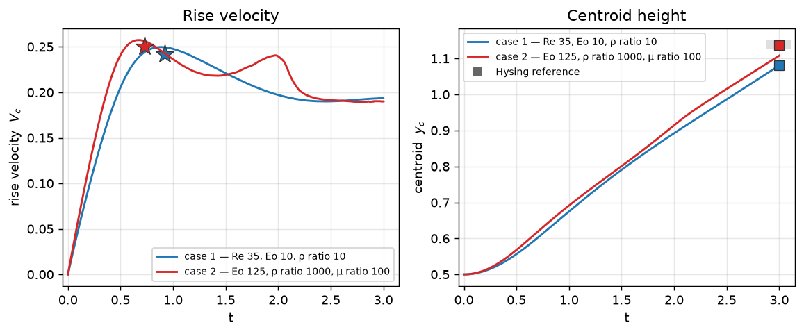
rows = []
for r in (r1, r2):
    p = r["p"]
    rows += [(f"case {r['case']}", "max rise velocity", r["vmax"], p["ref_vmax"],
              100 * (r["vmax"] / p["ref_vmax"] - 1)),
             (f"case {r['case']}", "y_c(3)", r["yc3"], p["ref_yc"],
              100 * (r["yc3"] / p["ref_yc"] - 1))]
print(f"{'':>7} {'quantity':>20} {'measured':>10} {'reference':>10} {'deviation':>10}")
for a, b, m, ref, d in rows:
    print(f"{a:>7} {b:>20} {m:10.4f} {ref:10.4f} {d:+9.1f} %")
quantity measured reference deviation
case 1 max rise velocity 0.2497 0.2417 +3.3 %
case 1 y_c(3) 1.0808 1.0810 -0.0 %
case 2 max rise velocity 0.2574 0.2502 +2.9 %
case 2 y_c(3) 1.1082 1.1376 -2.6 %Case 1’s centroid at \(t=3\) lands within 0.02 % of the published value and its peak rise velocity within 3.3 %. Case 2 reads 2.9 % and 2.6 % — inside the spread of the three reference codes themselves, on a case its authors describe as not grid-converged, at one resolution, with a periodic lateral condition standing in for free slip.
4. The shapes
fig, axes = plt.subplots(1, 6, figsize=(9.6, 4.4), sharey=True)
for j, (r, col) in enumerate(((r1, BLUE), (r2, RED))):
    nx = r["nx"]; sc = r["sc"]
    xg = (np.arange(nx) + 0.5) / sc.s
    zg = (np.arange(2 * nx) + 0.5) / sc.s
    for i, tt in enumerate(sorted(r["snaps"])):
        ax = axes[3 * j + i]
        B = r["snaps"][tt][:, 1, :]                     # mid-slab y-plane; B = bubble
        ax.set_facecolor("#eaf0f6")                     # the liquid
        ax.contourf(xg, zg, B.T, levels=[0.5, 1.5],     # the gas bubble
                    colors=["#fdf3ef" if r["case"] == 2 else "#eef6fd"])
        ax.contour(xg, zg, B.T, levels=[0.5], colors=[col], linewidths=1.8)
        ax.set(xlim=(0, 1), ylim=(0, 1.5), aspect="equal", xlabel="x",
               title=f"case {r['case']}, t = {tt:g}", xticks=[0, 0.5, 1])
        ax.grid(False)
axes[0].set_ylabel("y")
plt.tight_layout(); plt.show()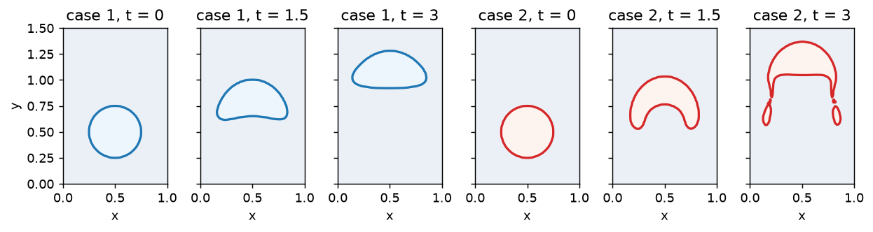
5. Momentum consistency is worth a factor five — at density ratio 10
enable_vof_momentum is the single most consequential option on this page. Repeat case 1 with it off, everything else identical:
r1_nc = hysing(1, momentum=False, snap_at=(0.0, 1.5, 3.0))
print(f"pressure {r1_nc['iters']}/{r1_nc['cap']} "
      f"{'OK' if r1_nc['iters'] < r1_nc['cap'] else '*** CAPPED -> INVALID ***'}, "
      f"max|div(open u)| {r1_nc['div']:.2e}, V(3)/V(0) = {r1_nc['vol'][-1]:.10f}\n")
p = HYSING[1]
print(f"{'case 1, ratio 10':>26} {'max V_c':>9} {'dev':>8}   {'y_c(3)':>8} {'dev':>8}")
for lab, r in (("momentum-consistent (on)", r1), ("inconsistent (off)", r1_nc)):
    print(f"{lab:>26} {r['vmax']:9.4f} {100*(r['vmax']/p['ref_vmax']-1):+7.1f}% "
          f"  {r['yc3']:8.4f} {100*(r['yc3']/p['ref_yc']-1):+7.1f}%")
print(f"{'reference (Hysing 2009)':>26} {p['ref_vmax']:9.4f} {'':>8}   {p['ref_yc']:8.4f}")
pressure 23/600 OK, max|div(open u)| 9.08e-06, V(3)/V(0) = 1.0000000000
case 1, ratio 10 max V_c dev y_c(3) dev
momentum-consistent (on) 0.2497 +3.3% 1.0808 -0.0%
inconsistent (off) 0.2827 +17.0% 1.2086 +11.8%
reference (Hysing 2009) 0.2417 1.0810fig, (axv, axy) = plt.subplots(1, 2, figsize=(9.0, 3.6))
for lab, r, col, ls in (("momentum-consistent", r1, BLUE, "-"),
("inconsistent", r1_nc, RED, "--")):
axv.plot(r["t"], r["vc"], ls, color=col, lw=1.7, label=lab)
axy.plot(r["t"], r["yc"], ls, color=col, lw=1.7, label=lab)
axv.plot(p["ref_tvmax"], p["ref_vmax"], "*", color="0.15", ms=15, label="Hysing reference")
axy.plot(3.0, p["ref_yc"], "s", color="0.15", ms=8, label="Hysing reference")
axv.set(xlabel="t", ylabel=r"rise velocity $V_c$", title="Rise velocity, case 1")
axy.set(xlabel="t", ylabel=r"centroid $y_c$", title="Centroid, case 1")
axv.legend(fontsize=8, loc="lower right"); axy.legend(fontsize=8, loc="upper left")
plt.tight_layout(); plt.show()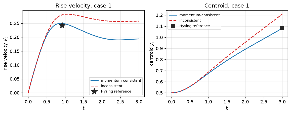
The inconsistent run misses the reference peak by 17.0 % and the centroid by 11.8 %, against 3.3 % and 0.02 % with consistency on — a factor five in the peak-velocity error and nearly three orders of magnitude in the centroid error, at density ratio 10. The literature’s rule of thumb is that consistent transport starts to matter around ratio 100–1000 (Rudman 1998); this says it is already paying for itself an order of magnitude earlier, on a benchmark where the reference is not in doubt.
Collocated cross-check
Since rung V8 the cell-centred grid (flow.SolverColocated) runs two-phase flow as well: variable density inside the approximate (ABC) projection — average the cell velocities onto a MAC face field, project that exactly, average the correction back — with buoyancy and surface tension applied as face accelerations and the cell taking the mean of its two faces, and with the colour advected by the projected face field. hysing() takes the solver class, so case 1 runs there with no other change.
One thing does not carry over, and it is the subject of §5: enable_vof_momentum is staggered-only. The consistent \(\rho\mathbf{u}\) transport needs Favre-averaged face states that the collocated construction does not have at this rung, and the call raises rather than quietly doing nothing. So the honest comparison is the momentum-consistency-off pair — the collocated run against r1_nc from §5, not against r1.
try:
    flow.SolverColocated(8, 8, 8).enable_vof_momentum(1.0, 10.0)
except RuntimeError as e:
    print(f"enable_vof_momentum on the collocated grid: RuntimeError\n  {str(e)[:160]}\n")

r1_co = hysing(1, momentum=False, cls=flow.SolverColocated, snap_at=(0.0,))
print(f"collocated: {r1_co['steps']} steps to t = 3, {r1_co['wall']:.0f} s, "
      f"pressure {r1_co['iters']}/{r1_co['cap']} "
      f"{'OK' if r1_co['iters'] < r1_co['cap'] else '*** CAPPED -> INVALID ***'}, "
      f"max|div(open u)| {r1_co['div']:.2e}, V(3)/V(0) = {r1_co['vol'][-1]:.10f}\n")
print(f"{'case 1, ratio 10, no momentum consistency':>42} {'max V_c':>9} {'t(peak)':>8} "
      f"{'y_c(3)':>9}")
for lab, r in (("staggered", r1_nc), ("collocated", r1_co)):
    print(f"{lab:>42} {r['vmax']:9.4f} {r['tvmax']:8.3f} {r['yc3']:9.4f}")
print(f"{'collocated vs staggered':>42} "
      f"{100*(r1_co['vmax']/r1_nc['vmax']-1):+8.2f}% {'':>8} "
      f"{100*(r1_co['yc3']/r1_nc['yc3']-1):+8.2f}%")
print(f"{'reference (Hysing 2009), for scale':>42} {p['ref_vmax']:9.4f} "
      f"{p['ref_tvmax']:8.3f} {p['ref_yc']:9.4f}")
enable_vof_momentum on the collocated grid: RuntimeError
enable_vof_momentum: momentum-consistent VoF transport is STAGGERED-ONLY (rung V2b); the collocated construction is Favre-averaged face states, rung V8.
peclet::flow SolverColocated: AUTO scheme fell back to gauge-exact (configuration unsupported by the ghost projection v1). Select explicitly with set_collocated_scheme to silence this notice.collocated: 2032 steps to t = 3, 339 s, pressure 23/600 OK, max|div(open u)| 9.12e-06, V(3)/V(0) = 1.0000000000
case 1, ratio 10, no momentum consistency max V_c t(peak) y_c(3)
staggered 0.2827 1.050 1.2086
collocated 0.2811 1.040 1.2132
collocated vs staggered -0.59% +0.38%
reference (Hysing 2009), for scale 0.2417 0.921 1.0810The two grids agree to 0.6 % on the peak rise velocity and 0.4 % on the centroid at \(t=3\), and both sit the same distance above the published curve — which is the point of the comparison. The gap to Hysing is not an artefact of the staggered mesh; it is the missing momentum consistency, worth a factor five here (§5), and it is missing on both grids in this table. Turning it back on is a staggered-only option today, so the collocated path’s honest rating for a case with motion is density ratio \(\lesssim 100\) — comfortable for case 1, not for case 2.
Adapt this yourself
- Refine.
hysing(1, nx=128)quadruples the cell count and shrinks the time step by \(h^{3/2}\) (the capillary limit) — the grid-convergence study the benchmark actually asks for. The interesting one is case 2, where the reference codes disagree. - Move in 3-D. Drop the quasi-2D slab: give \(y\) the same extent as \(x\) and initialise a sphere instead of a disc (
sphere_fractionsfrom the parasitic-currents page). Everything else is unchanged; the bubble is then a spherical cap and the rise velocity a different number. - Change the fluid pair. The
Scalemap takes physical SI numbers straight: an air bubble in water is \(\rho = 1.2/1000\), \(\mu = 1.8\!\times\!10^{-5}/10^{-3}\), \(\sigma = 0.072\) — ratio 830, and a good test of how far the momentum-consistent transport carries. - Add a wall or a packing.
set_solidputs SDF geometry in the box; the colour field is advected through it with openness-weighted geometric fluxes, which is the road from this page to a trickle-flow bed. - Go multi-rank. The identical script runs under
mpirun -np N python …;get_vof()/get_w()are collective gathers returning the field on rank 0.
Reproduce this
The compiled solver runs this, so its outputs are frozen into the site. To regenerate:
pip install peclet    # CPU wheels; for CUDA: pip install peclet-flow-cu13
quarto render examples/rising-bubble/index.qmd --execute
# ...or against a local source build of the suite (GPU):
PECLET_LOCAL_BUILD=/path/to/suite/flow/build_cuda OMP_NUM_THREADS=8 OMP_PROC_BIND=false \
  quarto render examples/rising-bubble/index.qmd --execute
The same two cases run inside the solver repo as tests/study/vof_surface_tension.py hysing1 hysing2.
References
Arrufat, T., M. Crialesi-Esposito, D. Fuster, et al. 2021. “A Mass-Momentum Consistent, Volume-of-Fluid Method for Incompressible Flow on Staggered Grids.” Computers & Fluids 215: 104785. https://doi.org/10.1016/j.compfluid.2020.104785.
Brackbill, J. U., D. B. Kothe, and C. Zemach. 1992. “A Continuum Method for Modeling Surface Tension.” Journal of Computational Physics 100 (2): 335–54. https://doi.org/10.1016/0021-9991(92)90240-Y.
Hysing, S., S. Turek, D. Kuzmin, et al. 2009. “Quantitative Benchmark Computations of Two-Dimensional Bubble Dynamics.” International Journal for Numerical Methods in Fluids 60 (11): 1259–88. https://doi.org/10.1002/fld.1934.
Rudman, Murray. 1998. “A Volume-Tracking Method for Incompressible Multifluid Flows with Large Density Variations.” International Journal for Numerical Methods in Fluids 28 (2): 357–78. https://doi.org/10.1002/(SICI)1097-0363(19980815)28:2<357::AID-FLD750>3.0.CO;2-D.