import importlib.util, os, subprocess, sys
_local = os.environ.get("PECLET_LOCAL_BUILD")
if _local:
    for p in _local.split(os.pathsep):
        sys.path.insert(0, p)
elif importlib.util.find_spec("peclet") is None:
subprocess.run([sys.executable, "-m", "pip", "install", "-q", "peclet"], check=True)Galilean invariance at finite Re: towed sphere vs fixed sphere
A sphere towed through fluid at rest and the same sphere held in a uniform stream are one physical problem in two frames. The solver’s moving-geometry machinery — fresh cells, wall velocity in the advection, the time term at a cut wall that moves — must reproduce the fixed-body answer step by step, and here it does, to 0.03 % at Re 1.5.
flow
IBM
moving-geometry
verification
exact
GPU
 GPU example — the frozen page reads correctly without a solver.
What you’ll learn
In a periodic box a uniform translation is an exact symmetry of the Navier–Stokes equations. So a sphere towed at speed \(U\) through fluid at rest and the same sphere fixed in a stream of speed \(U\) — started impulsively, with the same body force — must produce the same drag history at every step, not just the same steady value. The fixed case never touches the moving-geometry path; the towed case exercises all of it: the geometry rebuilt every step, cells that are uncovered and must be seeded, the wall velocity the advection operator must see inside the body, and the time term at a cut wall that is moving. Any gap between the two is a moving-geometry defect, cleanly separated from resolution (identical grids) and from confinement (identical images).
This is the finite-Reynolds-number extension of the Stokes Galilean gate the suite has carried since its moving-geometry rung landed — and the test that found, in 2026-08, that the advection operator was reading the solver’s masked zeros inside a moving body (zero is the wall velocity only for a wall that does not move). With that fixed, the pair below agrees to 0.03 % at Re 1.5 on the coarse grid, to 1 % on the finer one, and to 2 % at Re 30 — the residual in each case being the towed sphere’s cell-crossing oscillation around the same mean, not a drift.
Two solver hooks make the fixed twin possible: set_velocity(c, array) writes an initial field (a uniform stream), and set_body_force holds the box mean against the drag — the same value in both runs, because a body force is Galilean-invariant.
import time
import numpy as np
import matplotlib.pyplot as plt
from peclet import flow as sdflow
from peclet.core import geom

plt.rcParams.update({"figure.dpi": 130, "font.size": 9, "axes.axisbelow": True,
                     "figure.facecolor": "white", "savefig.bbox": "tight"})

U = 0.02           # tow / stream speed, cells per time unit
DT = 3.2
KI_I, KI_R = 2, 17
OFF = 0.3          # keep the sphere centre off the lattice


def abraham_cd(re):
    """Abraham (1970): C_D = 24/9.06^2 (9.06/sqrt(Re) + 1)^2 -- the standard-curve reference."""
    return 24.0 / 9.06 ** 2 * (9.06 / np.sqrt(re) + 1.0) ** 2
Kokkos::OpenMP::initialize WARNING: OMP_PROC_BIND environment variable not set
In general, for best performance with OpenMP 4.0 or better set OMP_PROC_BIND=spread and OMP_PLACES=threads
For best performance with OpenMP 3.1 set OMP_PROC_BIND=true
For unit testing set OMP_PROC_BIND=false
The pair
def make(N, DH, NU, y0):
    b = geom.SceneBuilder()
    sph = b.add_leaf("sphere", [DH / 2])
    ni, nr, _, _ = b.encode()
    ii = np.zeros((1, KI_I), dtype=np.int32); ir = np.zeros((1, KI_R))
    x0 = 0.5 * N + OFF
    ii[0] = (sph, -1); ir[0, 0:3] = (x0, y0, x0); ir[0, 6] = 1.0; ir[0, 7] = 1.0
    s = sdflow.Solver(N, N, N)
    s.set_rho(1.0); s.set_mu(NU); s.set_dt(DT); s.set_advection(True)
    s.set_velocity_solver_params(60); s.set_pressure_solver_params(20)
    s.set_pressure_multigrid(True, levels=4)
    s.set_scene(np.asarray(ni, np.int32), np.asarray(nr, float), ii.ravel(), ir.ravel(),
                periodic=True)
    s.set_solid_from_scene(True)
    return s, x0


def run(moving, N, DH, Re, steps):
    NU = U * DH / Re
    # The body force that holds the box mean: the Abraham drag at U per unit volume. The same
    # value in both runs; its mismatch with the true drag drifts the mean identically in both,
    # and the drift is measured below rather than assumed away.
    B = abraham_cd(Re) * 0.5 * U ** 2 * np.pi * (DH / 2) ** 2 / N ** 3
    y0 = 0.72 * N if moving else 0.5 * N + OFF
    s, x0 = make(N, DH, NU, y0)
    s.set_body_force(0.0, B, 0.0)
    if not moving:
        s.set_velocity(1, np.full((N, N, N), U, dtype=np.float64, order="F"))
    y = y0; F = []; t0 = time.time()
    for k in range(steps):
        if moving:
            s.set_instance_transform(0, [x0, y, x0])
            s.set_instance_motion(0, lin_vel=[0.0, -U, 0.0])
            s.rebuild_geometry()
        s.step()
        F.append(float(np.asarray(s.hydro_force_torque_reaction())[0][0][1]))
        if moving:
            y -= U * DT
    vmean = float(np.asarray(s.get_v()).mean()) / (1.0 - np.pi / 6 * DH ** 3 / N ** 3)
    urel = (U + vmean) if moving else vmean          # relative speed the sphere actually sees
    return np.array(F), urel, time.time() - t0
STEPS = 800
CASES = [(96, 8.0, 1.5), (96, 8.0, 30.0), (144, 12.0, 1.5)]
res = {}
print(" N d/h Re | F_fixed F_towed towed/fixed | step-by-step max |dF|/F | Cd/Abraham fixed towed | time")
for N, DH, Re in CASES:
Ff, uf, tf = run(False, N, DH, Re, STEPS)
Fm, um, tm = run(True, N, DH, Re, STEPS)
n4 = STEPS * 3 // 4
ff, fm = Ff[n4:].mean(), Fm[n4:].mean()
stepwise = np.abs(Fm[20:] - Ff[20:]).max() / np.abs(Ff[20:]).max()
cd = lambda f, u: f / (0.5 * u ** 2 * np.pi * (DH / 2) ** 2)
ref = lambda u: abraham_cd(u * DH / (U * DH / Re))
res[(N, DH, Re)] = dict(Ff=Ff, Fm=Fm, ratio=fm / ff, stepwise=stepwise,
cdf=cd(ff, uf) / ref(uf), cdm=cd(fm, um) / ref(um))
print(" %3d %4.1f %4.1f | %.5e %.5e %.4f | %.3f | %.4f %.4f | %4.0f s"
% (N, DH, Re, ff, fm, fm / ff, stepwise, res[(N, DH, Re)]["cdf"], res[(N, DH, Re)]["cdm"], tf + tm)) N d/h Re | F_fixed F_towed towed/fixed | step-by-step max |dF|/F | Cd/Abraham fixed towed | time
96 8.0 1.5 | 1.96098e-01 1.96152e-01 1.0003 | 0.004 | 0.9469 0.9472 | 331 s
96 8.0 30.0 | 2.13138e-02 2.08570e-02 0.9786 | 0.051 | 1.0303 1.0082 | 340 s
144 12.0 1.5 | 4.53907e-01 4.49786e-01 0.9909 | 0.007 | 0.9751 0.9660 | 628 sCode
fig, axes = plt.subplots(1, 2, figsize=(7.6, 3.0))
for ax, key in zip(axes, [(96, 8.0, 1.5), (96, 8.0, 30.0)]):
    r = res[key]; t = np.arange(1, STEPS + 1) * DT * U / key[1]
    ax.plot(t, r["Fm"], color="#4c72b0", lw=1.3, label="towed (moving geometry)")
    ax.plot(t, r["Ff"], color="#c44e52", lw=1.0, ls="--", label="fixed, stream U")
    ax.set_title("Re = %g,  d/h = %g" % (key[2], key[1]), fontsize=9)
    ax.set_xlabel("t U / d"); ax.set_xlim(0, t[-1]); ax.grid(alpha=0.3)
    lo = min(r["Fm"][100:].min(), r["Ff"][100:].min()); hi = max(r["Fm"][100:].max(), r["Ff"][100:].max())
    ax.set_ylim(lo - 0.15 * (hi - lo) - 1e-12, hi + 0.35 * (hi - lo) + 1e-12)
axes[0].set_ylabel("F_y (reaction)"); axes[0].legend(fontsize=8, frameon=False)
plt.show()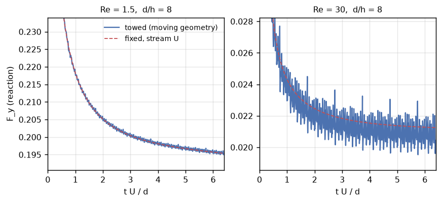
Results
| claim | measured | reference |
|---|---|---|
| towed / fixed quasi-steady drag, Re 1.5, d/h 8 | 1.0003 | 1 (exact symmetry) |
| step-by-step max deviation, Re 1.5 | 0.004 | 0 |
| towed / fixed, Re 1.5, d/h 12 | 0.9909 | 1 |
| towed / fixed, Re 30, d/h 8 | 0.9786 | 1, within the crossing oscillation |
| \(C_d\) / Abraham, fixed sphere, Re 1.5, d/h 8 → 12 | 0.947 -> 0.975 | 1 minus the periodic images (a few %) |
| \(C_d\) / Abraham, Re 30, d/h 8 | 1.030 | 1 |
The pair agrees to 0.03% at Re 1.5 on the coarse grid, 0.9% on the finer one, and 2.1% at Re 30 — in every case inside the amplitude of the towed sphere’s crossing oscillation, which averages out over many crossings but sets the floor of any single quasi-steady mean. What the pair does not test is the drag’s absolute accuracy: both members share the grid and the periodic images, and both sit a few percent from Abraham at \(d/h = 8\) for those two reasons. That is the point of the construction — it isolates the moving-boundary machinery from everything else, and finds nothing.
NoteWhy this gate exists
The Stokes version of this test has been in the suite since moving geometry landed. Its finite-Re extension was written in 2026-09 while chasing a confined-settling benchmark that missed by 18 %, to decide whether the moving boundary itself was at fault. It was not — the towed and fixed spheres agreed to 0.03 % — which sent the search elsewhere and found the real cause in a container built wider than its periodic box (see the settling sphere page). A gate that passes is as useful as one that fails, provided it is sharp enough to have failed.
Adapt this yourself
- Accelerate it. Replace the constant tow by a ramp \(U(t)\) and compare with the fixed sphere in a ramped stream (
set_velocityeach step is wasteful; a ramped body force is the clean twin) — the added-mass and history forces must match too. - Rotate it.
set_instance_motion(0, ang_vel=…)on the towed sphere against a fixed sphere with a rotating no-slip datum: the transposed-traction torque term is on the same footing. - Refine the towed side only. The pair must keep agreeing as \(\Delta t\) shrinks; the crossing oscillation at Re 30 should shrink with the Stokes-layer resolution, not with \(\Delta t\).
Reproduce this
PECLET_LOCAL_BUILD=/path/to/suite/flow/build_l3_cuda:/path/to/suite/core/python/build_geom \
  quarto render examples/galilean-drag/index.qmd --execute