import importlib.util, os, subprocess, sys
_local = os.environ.get("PECLET_LOCAL_BUILD")
if _local:
    for p in _local.split(os.pathsep):
        sys.path.insert(0, p)
elif importlib.util.find_spec("peclet") is None:
subprocess.run([sys.executable, "-m", "pip", "install", "-q", "peclet"], check=True)Torque on a rotating sphere: a negative result, then a fix
The Stokes torque 8πμa³Ω is exact and the geometry never moves — the cleanest possible torque test. peclet.flow failed it by a structural 31%, the cause turned out to be derivable in three lines, and the fix is a closed-form wall term with no reconstruction in it.
flow
IBM
verification
analytic
torque
GPU
 GPU example — the frozen page reads correctly without a solver.
What you’ll learn
A sphere of radius \(a\) spinning at angular velocity \(\Omega\) in unbounded quiescent Stokes flow feels
\[ \mathbf{T} = -8\pi\mu a^{3}\,\boldsymbol\Omega , \tag{1}\]
exactly — no series, no fitted constant. And a sphere is invariant under rotation about its own axis, so the geometry never moves: no fresh cells, no rebuild, none of the moving-boundary machinery. That makes this the sharpest torque test a resolved solver can face.
When this page was first written, peclet.flow failed it by 31% — structurally, in a way no refinement touched — while computing the force on the same runs to \(10^{-13}\). This page keeps that measurement, because how the failure was pinned down is the useful part; then it derives the cause exactly, applies the fix, and gates it. The one-sentence version: the missing torque was the transposed velocity gradient’s wall traction, it equals \(\mu\,(\mathbf n\times\boldsymbol\Omega)\) pointwise on a rigid rotating wall, its force integral is zero — which is why no force gate ever saw it — and it carries exactly one third of Equation 1.
The measurement that started it
The discrete-reaction route (hydro_force_torque_reaction) takes the force from the momentum the fluid actually lost. Per fluid cell \(R_i = -\nabla\pi_i + F_{\text{wall},i}\); summed over a body’s owner region the \(\nabla\pi\) telescopes away, and the force identity is gated elsewhere to \(-8.8\times10^{-15}\). The torque takes the first moment of the same data. Measured against Equation 1, before the fix (peclet-flow 1a01769, the recorded numbers):
| \(N\) | \(R/h\) | \(c\) | reaction torque error | net force \(/\mu R^2\Omega\) |
|---|---|---|---|---|
| 64 | 9.6 | 1.4e-02 | −30.54% | 5e-13 |
| 96 | 9.6 | 4.2e-03 | −31.58% | 3e-13 |
| 128 | 9.6 | 1.8e-03 | −31.82% | 4e-14 |
| 96 | 14.4 | 1.4e-02 | −31.04% | 2e-12 |
| 128 | 19.2 | 1.4e-02 | −31.00% | 1e-13 |
A factor of eight in box volume, 3.4 in solid fraction, two in \(R/h\), and 600 → 4000 steps: the deficit did not move. Not the periodic box (a periodic correction must vanish as \(c\to0\)), not the grid, not convergence — and the same runs get the force exactly right. A structural −31%.
The diagnosis, exact
The momentum operator discretises the Laplacian form \(\mu\nabla^2\mathbf u = \nabla\cdot(\mu\nabla \mathbf u)\), so the momentum the fluid loses through the wall is the Laplacian-form flux \(\mu\,\partial\mathbf u/\partial n\). The physical traction is \(\mu(\nabla\mathbf u + \nabla\mathbf u^{\mathsf T})\cdot\mathbf n\). The two differ by the transposed term — which vanishes in the interior for constant \(\mu\) and a solenoidal field (\(\nabla\cdot(\nabla\mathbf u^{\mathsf T}) = \nabla(\nabla\cdot\mathbf u) = 0\)), but not as a boundary traction.
Now the three lines. On a rigid no-slip wall moving with angular velocity \(\boldsymbol\Omega\), the fluid velocity equals the rigid-body field \(\mathbf u_w\), so all tangential derivatives of \(\mathbf u\) on the surface equal those of \(\mathbf u_w\) — and \(\nabla\mathbf u_w = [\boldsymbol\Omega\times]\), the constant spin tensor. Splitting the gradient into tangential and normal parts and using continuity (which kills the \(\mathbf n\,(\partial\mathbf u/\partial n \cdot \mathbf n)\) piece, because the spin tensor is traceless on the tangent plane):
\[ (\nabla\mathbf u)^{\mathsf T}\cdot\mathbf n \;=\; \mathbf n\times\boldsymbol\Omega \qquad\text{pointwise on the wall, exactly.} \tag{2}\]
No interior information whatsoever — only the wall’s own angular velocity and the local normal. Three consequences, each checkable:
- Force: \(\oint \mu(\mathbf n\times\boldsymbol\Omega)\,\mathrm dA = \mu\left(\oint\mathbf n\,\mathrm dA\right)\times\boldsymbol\Omega = 0\) over any closed surface. The force identity was never wrong, and no force-based validation could ever have caught this.
- Torque: \(\oint a\mathbf n\times\mu(\mathbf n\times\boldsymbol\Omega)\,\mathrm dA = -\tfrac{8\pi}{3}\mu a^3\boldsymbol\Omega\) — exactly one third of Equation 1. Predicted deficit −33.3%, measured −31.0%, the gap being discretisation.
- Translation: \(\boldsymbol\Omega = 0 \Rightarrow\) nothing. Every settling and drag result was always clean.
Equation 2 was verified against the analytic rotlet to \(3\times10^{-11}\) pointwise before anything was implemented. And it is not a novel observation: Maitri et al. (2018) measured the same resolution-independent 33–34% plateau on the IBM of Deen et al. (2012), which omits the same term, with the stated cause that the transposed terms carry a third of the analytic torque.
The fix
Since Equation 2 needs only wall kinematics and geometry, the correction is a closed-form surface integral over the cut cells,
\[ \Delta\mathbf T \;=\; \mu \sum_{\text{cut cells}} \mathbf r \times \left(\mathbf n\,\mathrm dA \times \boldsymbol\Omega\right), \tag{3}\]
with \(\mathbf n\,\mathrm dA\) the exact aperture wall-area vector the solver already carries. No near-wall velocity gradient, no reconstruction, no new field — the ingredients that made the traction route unreliable never enter. It is identically zero when nothing rotates, so every existing result is bit-identical, and the force is deliberately left untouched (adding a discretely zero term would only inject rounding into an identity gated at \(10^{-15}\)).
import time
import numpy as np
import matplotlib.pyplot as plt
from peclet import flow as sdflow

plt.rcParams.update({"figure.dpi": 130, "font.size": 9, "axes.axisbelow": True,
                     "figure.facecolor": "white", "savefig.bbox": "tight"})
RHO, MU = 1.0, 0.1
KN_R, KI_I, KI_R = 16, 2, 17
OMEGA = 1e-3
Kokkos::OpenMP::initialize WARNING: OMP_PROC_BIND environment variable not set
In general, for best performance with OpenMP 4.0 or better set OMP_PROC_BIND=spread and OMP_PLACES=threads
For best performance with OpenMP 3.1 set OMP_PROC_BIND=true
For unit testing set OMP_PROC_BIND=false
def spin(N, R, steps=1000, dt=20.0):
    x0 = 0.5 * N
    node_ints = np.array([1, -1, -1], dtype=np.int32)
    node_reals = np.zeros(KN_R); node_reals[0] = R
    node_reals[14] = 1.0; node_reals[15] = 1.0
    inst_ints = np.zeros((1, KI_I), dtype=np.int32); inst_ints[0] = (0, -1)
    inst_reals = np.zeros((1, KI_R)); inst_reals[0, 0:3] = (x0, x0, x0)
    inst_reals[0, 6] = 1.0; inst_reals[0, 7] = 1.0
    s = sdflow.Solver(N, N, N)
    s.set_rho(RHO); s.set_mu(MU); s.set_dt(dt)
    s.set_advection(False)
    s.set_velocity_solver_params(100); s.set_pressure_solver_params(25)
    s.set_pressure_multigrid(True, levels=4)
    s.set_scene(node_ints, node_reals, inst_ints.ravel(), inst_reals.ravel(), periodic=True)
    s.set_instance_motion(0, lin_vel=[0, 0, 0], ang_vel=[0, 0, OMEGA], center=[x0, x0, x0])
    s.set_solid_from_scene(True)
    t0 = time.time()
    for _ in range(steps):
        s.step()
    react = np.asarray(s.hydro_force_torque_reaction())
    exact = 8 * np.pi * MU * R ** 3 * OMEGA
    return dict(T=abs(react[1][0][2]), Texact=exact,
                Fnet=np.linalg.norm(react[0][0]) / (MU * R ** 2 * OMEGA),
                c=(4 / 3) * np.pi * R ** 3 / N ** 3, N=N, R=R, wall=time.time() - t0)
Step 1 — The same ladders, after the fix
BEFORE = {(64, 9.6): -30.54, (96, 9.6): -31.58, (128, 9.6): -31.82,
          (96, 14.4): -31.04, (128, 19.2): -31.00}
print("  N    R/h    c        T/T_exact - 1   (before the fix)   net force")
rows = []
for N, R in ((64, 9.6), (96, 9.6), (128, 9.6), (96, 14.4), (128, 19.2)):
    r = spin(N, R)
    rows.append(r)
    print("  %3d  %5.1f  %.1e     %+6.2f%%          (%+.2f%%)        %.1e   (%3.0f s)"
          % (N, R, r["c"], 100 * (r["T"] / r["Texact"] - 1), BEFORE[(N, R)], r["Fnet"],
             r["wall"]))
N R/h c T/T_exact - 1 (before the fix) net force
64 9.6 1.4e-02 +3.47% (-30.54%) 5.3e-13 ( 73 s)
96 9.6 4.2e-03 +2.42% (-31.58%) 2.8e-13 (114 s)
128 9.6 1.8e-03 +2.19% (-31.82%) 3.9e-14 (196 s)
96 14.4 1.4e-02 +2.89% (-31.04%) 1.5e-12 (114 s)
128 19.2 1.4e-02 +2.61% (-31.00%) 6.8e-14 (196 s)Code
fig, ax = plt.subplots(figsize=(6.2, 3.0))
lab = ["$N$=%d\n$R/h$=%.1f" % (r["N"], r["R"]) for r in rows]
x = np.arange(len(rows))
ax.bar(x - 0.18, [BEFORE[(r["N"], r["R"])] for r in rows], 0.34, color="0.75",
       label="before (recorded)")
ax.bar(x + 0.18, [100 * (r["T"] / r["Texact"] - 1) for r in rows], 0.34, color="#4c72b0",
       label="with the wall term")
ax.axhline(0, color="0.3", lw=1.0, ls="--")
ax.axhline(-100 / 3, color="#c44e52", lw=0.9, ls=":", label="−33.3% (the exact third)")
ax.set_xticks(x); ax.set_xticklabels(lab, fontsize=7.5)
ax.set_ylabel("error in $T_z$ vs $8\\pi\\mu a^3\\Omega$ [%]")
ax.legend(fontsize=8, frameon=False); ax.grid(axis="y", alpha=0.3)
plt.show()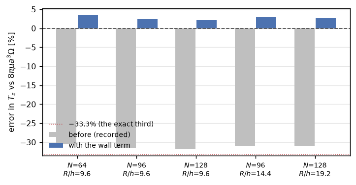
Two things to notice. The before-bars sit on the dotted line at −33.3% to within discretisation — the failure itself confirmed the diagnosis. And the after-bars converge: box growth moves 3.47% -> 2.42% -> 2.19% and grid refinement 2.89% -> 2.61%, tracking the solver’s own aperture first-moment accuracy — a discretisation error now, not a missing term.
Step 2 — The loop closed: a sphere that spins down
The point of the torque is the resolved CFD-DEM coupling. With apply_torque=True, ResolvedCfdDem hands the reaction torque to peclet.dem, which integrates Euler’s equations. A freely spinning sphere with physical inertia \(I = \tfrac{2}{5}mR^2\) must decay at the rate \(1/\tau = 8\pi\mu R^3\lambda_{\text{rot}}/I\), with \(\lambda_{\text{rot}}\) the same box’s own rotational drag from Step 1 — the calibration pattern that makes the discretisation bias cancel between calibration and prediction.
from peclet import dem as pdem
from peclet_coupling.resolved import ResolvedCfdDem

N, R, DT = 64, 9.6, 5.0
RHO_P = 5.0
m = RHO_P * 4 / 3 * np.pi * R ** 3
I = 0.4 * m * R ** 2
lam = rows[0]["T"] / rows[0]["Texact"]          # the same box's calibrated rotational drag
tau = I / (8 * np.pi * MU * R ** 3 * lam)
nstep = int(1.2 * tau / DT)
print("tau_pred = I / (8 pi mu R^3 lambda_rot) = %.1f   (%d coupled steps)" % (tau, nstep))

d = pdem.Simulation(8)
d.set_gravity(0.0, 0.0, 0.0)
d.set_sphere_shape(1.0)
d.set_global_scale(R)
d.set_positions(np.array([[0.5 * N, 0.5 * N, 0.5 * N]], dtype=np.float32))
d.set_inv_mass(np.array([1.0 / m], dtype=np.float32))
d.set_inv_inertia(np.array([[1.0 / I] * 3], dtype=np.float32))   # PHYSICAL inertia: mandatory
d.set_angular_velocities(np.array([[0.0, 0.0, OMEGA]], dtype=np.float32))

s = sdflow.Solver(N, N, N)
s.set_rho(RHO); s.set_mu(MU); s.set_dt(DT); s.set_advection(False)
s.set_velocity_solver_params(100); s.set_pressure_solver_params(25)
s.set_pressure_multigrid(True, levels=4)
drv = ResolvedCfdDem(s, d, radius=R, mu=MU, rho_f=RHO, fluid_dt=DT, dem_substeps=10,
                     periodic=True, rho_p=RHO_P, buoyancy=False, move=True, apply_torque=True)
ts, oms = [], []
for k in range(nstep):
    drv.step()
    ts.append((k + 1) * DT)
    oms.append(float(np.asarray(d.get_angular_velocities())[0, 2]))
ts = np.array(ts); oms = np.array(oms)
mfit = ts <= tau
rate = -np.polyfit(ts[mfit], np.log(oms[mfit] / OMEGA), 1)[0]
print("Omega fell to %.3f Omega0 over %.0f time units" % (oms[-1] / OMEGA, ts[-1]))
print("fitted decay rate x tau_pred = %.4f   (1 = the box's own calibrated drag)" % (rate * tau))
tau_pred = I / (8 pi mu R^3 lambda_rot) = 296.9 (71 coupled steps)Kokkos::OpenMP::initialize WARNING: OMP_PROC_BIND environment variable not set
In general, for best performance with OpenMP 4.0 or better set OMP_PROC_BIND=spread and OMP_PLACES=threads
For best performance with OpenMP 3.1 set OMP_PROC_BIND=true
For unit testing set OMP_PROC_BIND=false
Omega fell to 0.262 Omega0 over 355 time units
fitted decay rate x tau_pred = 1.0389   (1 = the box's own calibrated drag)
Code
fig, ax = plt.subplots(figsize=(5.6, 3.0))
ax.semilogy(ts / tau, oms / OMEGA, "o-", ms=3, color="#4c72b0", label="dem-integrated")
ax.semilogy(ts / tau, np.exp(-ts / tau), "--", color="#c44e52",
            label=r"$e^{-t/\tau}$, $\tau$ from the same box")
ax.set_xlabel(r"$t/\tau$"); ax.set_ylabel(r"$\Omega/\Omega_0$")
ax.legend(fontsize=8, frameon=False); ax.grid(which="both", alpha=0.3)
plt.show()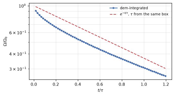
What is still not right
The reconstructed-traction torque (hydro_force_torque, the diagnostic route) has an unrelated defect this page found on the way: on a perfectly steady field it drifts linearly with step count, because the cut-cell pressure operator decouples solid-centred cells, nothing pins their value, the incremental scheme accumulates into them, and the surface integral samples them. Measured: std\((P)\) over fluid cells constant at \(7\times10^{-7}\); over solid cells linear, \(2.5\times10^{-4}
\to 1.6\times10^{-3}\) over 4000 steps, the traction torque tracking it from −26% to +83%. That route stays a diagnostic; the fix (pinning the decoupled gauge cells) is logged in the design note and deferred. Every coupling-facing quantity uses the reaction route.
Results
| claim | measured | reference |
|---|---|---|
| reaction torque, before the fix (recorded) | −31.0%, flat under all refinement | Equation 1 |
| the missing term, derived | \((\nabla\mathbf u)^{\mathsf T}\mathbf n = \mathbf n\times\boldsymbol\Omega\), verified to 3e-11 | exactly \(\tfrac13\) of the torque, 0 of the force |
| reaction torque, with the wall term | +3.47% / +2.42% / +2.19% — converging | Equation 1 |
| net force on the same runs | 2e-12 | 0 by symmetry |
| spin-decay through the full dem loop | rate × τ = 1.0389 | 1 (same-box calibration) |
| force gates after the change | bit-identical | — |
The headline: the torque went from a structural −31% to +2.19% and converging, with a correction derived in closed form rather than fitted — and the first freely rotating resolved particle in this suite decays at 1.039× its own box’s calibrated drag. The Jeffery orbit, blocked when this page was a pure negative result, is now buildable.
Adapt this yourself
- Keep it as a gate. Spin a sphere, compare to \(8\pi\mu a^3\Omega\), refine box and grid separately. Two ladders and an exact answer distinguish a bias from a bug — that recipe found this, diagnosed it, and verified the fix.
- Check your own solver for the same term. If your momentum equation is the Laplacian form and your force comes from a momentum budget, your torque is missing \(\mu(\mathbf n\times\boldsymbol\Omega)\) too — and no drag validation will ever show it.
- Free rotation, now.
set_inv_inertiawith the physical inertia, thenResolvedCfdDem(..., apply_torque=True). The inertia is mandatory: dem’s default is not your grain’s, and a torque against a wrong inertia spins up at an arbitrary rate.
Reproduce this
PECLET_LOCAL_BUILD=/path/to/suite/flow/build_l3_cuda:/path/to/suite/dem/build_l4_omp:/path/to/suite/coupling/python \
  quarto render examples/rotating-sphere-torque/index.qmd --execute
References
Deen, N. G., S. H. L. Kriebitzsch, M. A. van der Hoef, and J. A. M. Kuipers. 2012. “Direct Numerical Simulation of Flow and Heat Transfer in Dense Fluid–Particle Systems.” Chemical Engineering Science 81: 329–44.
Maitri, R. V., S. Das, J. A. M. Kuipers, J. T. Padding, and E. A. J. F. Peters. 2018. “An Improved Ghost-Cell Sharp Interface Immersed Boundary Method with Direct Forcing for Particle Laden Flows.” Computers & Fluids 175: 111–28. https://doi.org/10.1016/j.compfluid.2018.08.018.