import importlib.util, os, subprocess, sys
_local = os.environ.get("PECLET_LOCAL_BUILD")
if _local:
    for p in _local.split(os.pathsep):
        sys.path.insert(0, p)
elif importlib.util.find_spec("peclet") is None:
subprocess.run([sys.executable, "-m", "pip", "install", "-q", "peclet"], check=True)Navier–Stokes on a Voronoi mesh: the Taylor–Green vortex
Run peclet.voro’s two static flow solvers — the staggered covolume scheme and the collocated scheme with flow’s approximate projection — on an unstructured Voronoi mesh, and measure what each one gets right: exact energy conservation for one, second order for the other.
voro
flow
verification
unstructured
What you’ll learn
peclet.voro is a GPU Voronoi engine; since track C of its methods plan it also carries a finite-volume Navier–Stokes solver on the Voronoi face mesh. Two discretisations share one operator layer: the covolume scheme (face-normal fluxes, exact projection, exact discrete energy conservation) and the collocated scheme (seed velocities, peclet.flow’s approximate projection with the pressure gradient that is the exact transpose of the centre-to-face constraint). You’ll see why a Voronoi mesh is the natural mesh for a two-point flux — the seed connector is perpendicular to the face by construction — and what limits each scheme on an unstructured mesh. Headline: on a jittered lattice the collocated scheme converges at second order (the suite’s tests: 2.1 on jittered lattices, 2.1 on centroidal meshes) while the covolume scheme’s face flux is first order — its reconstructed cell velocity, shown here, does a little better — and the covolume scheme’s inviscid energy drift is purely the time-stepping error.
The problem
The 2-D Taylor–Green vortex extended uniformly along \(z\) is an exact solution of the 3-D incompressible Navier–Stokes equations in a periodic box of side \(L\), \(k = 2\pi/L\): \[ u = \sin kx\,\cos ky\; e^{-2\nu k^2 t},\qquad v = -\cos kx\,\sin ky\; e^{-2\nu k^2 t},\qquad w = 0, \tag{1}\] so its kinetic energy decays as \(E(t)/E(0) = e^{-4\nu k^2 t}\) and the velocity field itself is known at every time — the reference for both a decay-rate check and a convergence study. The mesh is the Voronoi tessellation of a cubic lattice of seeds jittered by \(\pm0.2\,h\): a genuinely unstructured mesh (the unjittered lattice is degenerate, eight cells meeting at every vertex).
import numpy as np
import matplotlib.pyplot as plt
from peclet import voro
from peclet_examples.voro_flow import jittered_lattice, taylor_green
plt.rcParams.update({"figure.dpi": 130, "font.size": 10, "axes.grid": True, "grid.alpha": 0.3})
print("peclet.voro execution space:", voro.execution_space)
peclet.voro execution space: OpenMPBuild the mesh, run both solvers
A Tessellation holds the resident Voronoi cells; a FlowSolver builds the face mesh from it (one record per geometric face: owner, neighbour, area, connector) and steps the flow. Both layouts take the same initial field, a body force, a viscosity — here \(\nu = 0.01\), so \(\mathrm{Re} = UL/\nu = 100\) — and SSP-RK3 with a pressure projection per stage.
n, L, nu = 16, 1.0, 0.01
pos = jittered_lattice(n, L, jitter=0.2, seed=3)
t = voro.Tessellation()
t.set_box((L, L, L))
t.build(pos)
k = 2 * np.pi / L
T, dt = 0.25, 0.2 * L / n            # CFL 0.2 on the seed spacing
steps = int(np.ceil(T / dt))
runs = {}
for layout in ("covolume", "collocated"):
    f = voro.FlowSolver(t, nu, layout=layout)
    f.set_velocity(taylor_green(pos, 0.0, nu, L))
    E0, E, times = f.kinetic_energy(), [1.0], [0.0]
    for s in range(steps):
        f.step(1, T / steps)
        E.append(f.kinetic_energy() / E0); times.append((s + 1) * T / steps)
    U = f.get_velocity()
    Uex = taylor_green(pos, T, nu, L)
    err = np.sqrt(np.sum((U - Uex) ** 2 * f.get_cell_volume()[:, None]) / np.sum(Uex ** 2 * f.get_cell_volume()[:, None]))
    runs[layout] = dict(times=np.array(times), E=np.array(E), err=err, div=f.max_divergence())
    print(f"{layout:11s}: E/E0 = {E[-1]:.5f} (exact {np.exp(-4 * nu * k * k * T):.5f}), "
          f"cell-velocity error {err:.3e}, max face divergence {runs[layout]['div']:.1e}")
covolume : E/E0 = 0.68555 (exact 0.67383), cell-velocity error 2.935e-02, max face divergence 9.4e-14
collocated : E/E0 = 0.67523 (exact 0.67383), cell-velocity error 2.982e-02, max face divergence 9.1e-15Both track the analytic decay; the transporting face flux is divergence-free to round-off in both schemes (the covolume scheme projects its face field exactly; the collocated scheme projects the face average of the cell field exactly — that is the “approximate” of the approximate projection).
fig, ax = plt.subplots(figsize=(5.5, 3.6))
tt = runs["covolume"]["times"]
ax.plot(tt, np.exp(-4 * nu * k * k * tt), "k-", lw=2, label="exact")
for layout, st in (("covolume", "o"), ("collocated", "s")):
    ax.plot(runs[layout]["times"][::6], runs[layout]["E"][::6], st, ms=4, label=layout)
ax.set(xlabel="t", ylabel="E(t)/E(0)"); ax.legend()
plt.show()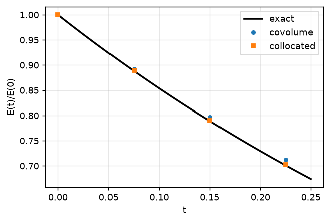
Convergence on an unstructured mesh
Now the point of the example. Refine the jittered lattice (\(n = 8, 16, 24\)) and measure the cell-velocity error at \(t = T\) for both schemes.
def tgv_error(layout, n, nu=0.01, L=1.0, T=0.25):
    pos = jittered_lattice(n, L, jitter=0.2, seed=n)
    t = voro.Tessellation(); t.set_box((L, L, L)); t.build(pos)
    f = voro.FlowSolver(t, nu, layout=layout)
    f.set_velocity(taylor_green(pos, 0.0, nu, L))
    steps = int(np.ceil(T / (0.2 * L / n)))
    f.step(steps, T / steps)
    U, Uex, V = f.get_velocity(), taylor_green(pos, T, nu, L), f.get_cell_volume()[:, None]
    return np.sqrt(np.sum((U - Uex) ** 2 * V) / np.sum(Uex ** 2 * V))

ns = [8, 16, 24]
errs = {layout: [tgv_error(layout, n) for n in ns] for layout in ("covolume", "collocated")}
for layout in errs:
    e = errs[layout]
    orders = [np.log(e[i] / e[i + 1]) / np.log(ns[i + 1] / ns[i]) for i in range(len(ns) - 1)]
    print(f"{layout:11s}: errors {['%.3e' % x for x in e]}  orders {['%.2f' % o for o in orders]}")
covolume : errors ['1.062e-01', '2.961e-02', '1.404e-02'] orders ['1.84', '1.84']
collocated : errors ['9.996e-02', '2.941e-02', '1.257e-02'] orders ['1.76', '2.10']fig, ax = plt.subplots(figsize=(5, 3.6))
h = 1.0 / np.array(ns)
for layout, st in (("covolume", "o-"), ("collocated", "s-")):
ax.loglog(h, errs[layout], st, label=layout)
ax.loglog(h, errs["collocated"][0] * (h / h[0]) ** 2, "k--", lw=1, label="h²")
ax.loglog(h, errs["covolume"][0] * (h / h[0]), "k:", lw=1, label="h")
ax.set(xlabel="seed spacing h", ylabel="relative L2 error"); ax.legend()
plt.show()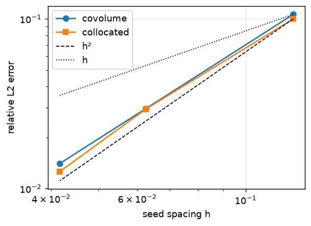
Why
- A Voronoi face is the perpendicular bisector of its seed connector, so the two-point flux \((p_j - p_i)\,A_{ij}/d_{ij}\) is consistent with no non-orthogonal correction, and the pressure Laplacian is the graph Laplacian \(A/d\) — the same matrix the Voronoi optimiser assembles.
- The only mesh-quality error left is skewness: the face centroid sits off the connector. The collocated scheme’s centre-to-face constraint extrapolates each cell to the face centroid with a Green–Gauss gradient corrected by the per-cell Gauss identity \((I - S)^{-1}\), \(S = \tfrac{1}{V}\sum_f A_f\, t_f \otimes n_f\) — exact for linear fields on any polyhedron — and the cell pressure gradient is the exact transpose of that constraint. That pair is what makes it second order on this mesh.
- The covolume scheme reconstructs the cell velocity from the fluxes with the Perot formula, which is only first-order consistent on non-symmetric cells; its viscous term inherits that. Its strength is structural: the face momentum operator is the exact adjoint of the reconstruction, so the semi-discrete scheme conserves \(\tfrac12\langle u,u\rangle_F\) exactly in the inviscid limit (the measured drift is the RK3 time error, order 2.96 in \(\Delta t\)).
Adapt this yourself
- Lloyd-relax the seeds first (
t.energy_forces(..., lloyd=1.0)gives the centroidal gradient): skewness drops from 0.08 to 0.04 and both errors shrink; the covolume scheme reaches order ≈ 1.3 on a centroidal mesh. - Add walls: give the tessellation an SDF (
t.set_geometry) and the sameFlowSolvertreats the clipped faces as no-slip walls — see the sphere-drag example. - Go implicit:
f.set_implicit_diffusion(True)is flow’s semi-implicit step (explicit convection, backward-Euler viscous solve, approximate projection); it removes the diffusive step limit for creeping flows. - Go multi-rank: the same solver runs distributed over
VoronoiHalo(C++ today;tests/kokkos_mpi/test_flow_mpi), np = 2/4 agree with a single rank to 3e-15.
Reproduce this
pip install -e .          # + a recent peclet (peclet-voro with FlowSolver)
quarto render examples/voronoi-taylor-green/index.qmd --execute
# local suite build instead of PyPI (the voro build dir with the Python module):
PECLET_LOCAL_BUILD=/path/to/suite/voro/build_a0 quarto render examples/voronoi-taylor-green/index.qmd --execute