Peclet

A suite of GPU-accelerated and parallel codes for the simulation of transport phenomena — Eulerian (CFD / Navier–Stokes, single- and two-phase), Lagrangian (DEM / granular dynamics), mixed (Voronoi) and coupled (CFD-DEM) methods, sharing one MPI block domain decomposition with asynchronous ghost-layer exchange, SDF-described solids, a common immersed-boundary methodology, GPU support (Kokkos: CUDA / HIP / OpenMP), and Python bindings everywhere.

The name nods to the Péclet number — the ratio of advective to diffusive transport, the dimensionless heart of transport phenomena.

Watch: the 1.1.0 release film

Eight minutes on what the suite does and, at length, the evidence for it — the exact solutions first, then published experiments, then the release's own scaling record: 32 H100 GPUs carrying 1.81 billion cells at 64 % weak efficiency, every rung returning the same mean velocity to one part in ten billion. It is also open about how it was built.

Watch on YouTube · the channel @PecletHPC carries a short movie for every example in the gallery, each one linking back to the page that produced it.

Quick start (Python)

The codes are driven from Python — one peclet.* namespace, installable from PyPI. The multicore-CPU (OpenMP) build ships as self-contained wheels, and so does the single-GPU CUDA build:

pip install peclet          # CPU family: peclet-morton + peclet-flow + peclet-pnm + peclet-dem + peclet-voro
pip install peclet-cu13     # the same family as CUDA wheels (NVIDIA driver only; not alongside `peclet`)
pip install peclet-flow     # or any single package

Wheels cover Linux (x86-64 and aarch64), Windows x64 and macOS on Apple silicon, CPython 3.10–3.14, all multi-threaded — OpenMP on Linux, Kokkos' C++ threads backend on the other two, since neither of those toolchains supplies an OpenMP that Kokkos accepts (DEPLOYMENT.md). A GPU on Windows means WSL2. The Colab link below needs nothing installed at all.

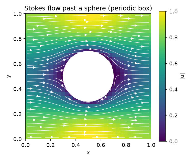
Stokes flow past a sphere in a box of side L, start to finish: 2.5 s on two workstation cores, around half a minute on the two shared vCPUs of a free Colab runtime (it prints its own wall clock). The physical problem is stated in your own units and N sets the resolution, so a grid-refinement study is one number away — at a price: N = 48 is eight times the work of N = 32. Run it as is, or open the same steps as a notebook in Colab — the first cell installs the wheels:

import time

import numpy as np
import peclet.flow as flow

# --- the physical problem, in any consistent unit system -------------------------------------
L, R = 1.0, 0.2              # side of the periodic box and radius of the sphere at its centre
rho, mu = 1.0, 0.1           # fluid density and viscosity
F = 1.0                      # driving pressure gradient along x (force per unit volume)
N = 32                       # cells per side: change this for a grid-refinement study

s = flow.Solver((N, N, N), extent=(L, L, L))                    # a periodic box: a cubic lattice of spheres
s.set_rho(rho); s.set_mu(mu); s.set_dt(1e3)                    # every input physical; a large dt marches
s.set_body_force((F, 0.0, 0.0))                                #   straight to the steady Stokes flow

x, y, z = s.cell_centers()                                     # the grid the solver laid inside the box
X, Y, Z = np.meshgrid(x, y, z, indexing="ij")
sdf = np.sqrt((X - L/2)**2 + (Y - L/2)**2 + (Z - L/2)**2) - R  # signed distance, < 0 inside the sphere
s.set_solid(sdf, cutcell_pressure=True)                        # no-slip cut-cell immersed boundary

t0, u_mean = time.perf_counter(), []
for it in range(200):
    s.step()
    u_mean.append(s.get_u().mean())
    if it >= 3 and abs(u_mean[-1] - u_mean[-4]) < 1e-3 * abs(u_mean[-1]):
        break                                                  # steady: three steps have not moved it
u, v, w = s.get_u(), s.get_v(), s.get_w()                      # physical velocity, physical pressure
p = s.get_p()
k = mu * u.mean() / F                                          # Darcy permeability of the sphere lattice
print(f"{flow.execution_space}: N = {N}, {it + 1} steps, {time.perf_counter() - t0:.1f} s, "
      f"permeability k = {k:.4e}")

# --- a look at the flow: speed and streamlines on the mid-plane through the sphere ---------------
import matplotlib.pyplot as plt
c = N // 2
speed = np.hypot(u[:, :, c], v[:, :, c])
plt.figure(figsize=(5, 4.2))
plt.imshow(speed.T, origin="lower", cmap="viridis", extent=[0, L, 0, L])
plt.streamplot(x, y, u[:, :, c].T, v[:, :, c].T, color="w", density=1.2, linewidth=0.6)
th = np.linspace(0, 2 * np.pi, 180)                             # the sphere itself, drawn exactly
plt.fill(L/2 + R*np.cos(th), L/2 + R*np.sin(th), color="w", zorder=3)
plt.colorbar(label="|u|"); plt.title("Stokes flow past a sphere (periodic box)")
plt.xlabel("x"); plt.ylabel("y"); plt.tight_layout()
plt.show()

Running this in a container? Bound the thread pool first.

Kokkos sizes its OpenMP pool from the CPUs it can see. Colab, Binder, Docker and a Slurm cgroup all normally show you the whole host while granting a fraction of it, so the default pool spin-waits itself to a standstill — measured on the wheel above, this 2.5-second solve did not finish in 15 minutes on 2 CPUs of quota with 48 visible, and took 2.5 s with the pool bounded. Before importing peclet:

import os
os.environ.setdefault("OMP_NUM_THREADS", "2")   # or however many CPUs you were actually granted
os.environ.setdefault("OMP_PROC_BIND", "false")

The Colab notebook linked above resolves this process's own cgroup and takes the tightest quota on the chain — /sys/fs/cgroup/cpu.max is the cgroup root, and reads max on a host that does limit you. On a workstation you do not need it: there, visible and granted are the same.

→ Examples gallery (runnable, validated notebooks) · Python API reference · Install & run (GPU / MPI / HPC containers).

The codes

Code	PyPI · import	Role
geom	peclet-geom · peclet.geom	Analytic-SDF scene authoring: CSG trees, batch evaluation, lattice baking, rigid-body mass properties. Host-only — wheels, numpy the only dependency, included in pip install peclet
core	peclet-halo · peclet.halo	Shared infrastructure: ORB block decomposition, async grid/particle halo, migration and rebalancing, sampled SDF geometry, VTI I/O. The C++ headers remain peclet/core/…; the Python distribution is peclet-halo
flow	peclet-flow · peclet.flow	Incompressible Navier–Stokes for porous media (staggered MAC or collocated grid, cut-cell IBM, multigrid), geometric VoF two-phase flow, moving analytic geometry
pnm	peclet-pnm · peclet.pnm	Pore-network extraction from SDF geometry (pores, watershed segmentation, throat topology) and network flow data from a flow DNS
dem	peclet-dem · peclet.dem	Discrete Element Method (XPBD and Hertz–Mindlin) with SDF point-shell collision for spheres and arbitrary SDF shapes
voro	peclet-voro · peclet.voro	Dynamic 3D Voronoi tessellation of moving particles (periodic boxes), mesh generation, Navier–Stokes on a Voronoi mesh
coupling	peclet-coupling · peclet.coupling	CFD-DEM: unresolved (volume-averaged drag) and resolved (cut-cell) two-way coupling of flow and dem
morton	peclet-morton · peclet.morton	Morton/Z-order codes with arithmetic in Morton space — the spatial-index primitive

The GPU codes are Kokkos-based: the same source runs on CUDA, HIP (AMD/LUMI) and OpenMP, chosen at build time by the install prefix, the wheel flavour (peclet vs peclet-cu13) or the container.

Examples gallery

computational-chemical-engineering.github.io/peclet-examples is the worked-examples site: every page is a notebook executed against the released package, with an Open in Colab button and the validation numbers in the open —

• Single-phase flow — exact and canonical benchmarks (Poiseuille, Taylor–Green, lid-driven cavity, Schäfer–Turek cylinder, Rayleigh–Bénard, turbulent channel DNS) and moving-body drag / torque cases.
• Packings & porous media — Zick–Homsy sphere arrays, random and ring packed beds (dem → flow), pore-space Voronoi meshes, pore-network extraction.
• Two-phase flow (VoF) — advection benchmarks, parasitic currents, capillary waves, rising bubble, wetting, bubbles and trickle flow through packings.
• Granular (DEM) — SDF-shaped particles, rotating drum, tumbling cubes, Pall rings, stirred column.
• CFD-DEM — fluidized bed, bubble injection, segregation, homogeneous cooling (MFIX-Exa comparisons).
• Benchmarks — the multi-GPU and CPU scaling studies (Snellius) and a DEM bulk-flow benchmark.

Where a page has a movie, the movie is on @PecletHPC — a bubble squeezing through a packed bed, a million-particle fluidized bed, tumbling cubes in a drum, Rayleigh–Bénard convection, trickle flow over a packing, the tennis-racket effect — and each video's description links straight back to the page with the code and the numbers.

Documentation

• Examples gallery — start here if you want to use the suite.
• Videos (@PecletHPC) — the 1.1.0 release film and a movie for every example that has one.
• Python API reference — the classes and methods you call from Python (the primary interface).
• Install & run — the backend × MPI matrix, pip install recipes (CPU wheels, CUDA wheels, source builds) and the HPC routes.
• Containers (HPC) — pull the pre-built Apptainer images from GHCR (or build your own) and run on a laptop, Snellius, or LUMI.
• Snellius · LUMI — the site runbooks.
• Architecture · Conventions · Interfaces · Roadmap — the cross-cutting design contract.
• C++ API (Doxygen) — the full C++ API per code: core · morton · flow · pnm · dem · voro
• Changelog — what each family release contains; the PyPI badge above shows the current version.

Citing

If you use Peclet in your research, please cite it. Each release is archived on Zenodo:

• Concept DOI (all versions): 10.5281/zenodo.21132445 — always resolves to the latest release; use this unless you need to pin an exact version.
• A specific version: the Zenodo record above lists a version DOI for every release, and each GitHub release links to its own.

Machine-readable metadata lives in CITATION.cff — use GitHub's "Cite this repository" button for ready-made BibTeX/APA.