Staggered vs collocated flow: grid-convergence, accuracy & performance¶
Source
Generated by flow/tests/study/staggered_vs_colocated.py; the canonical copy lives in the flow
submodule at flow/doc/history/colocated_study/. Reproduce with that script's run / report modes.
Primary backend: gpu (Cuda). Second backend: cpu-omp16. Both solvers share every operator (cut-cell IBM, geometric pressure multigrid, rotational pressure, MPI); they differ only in velocity placement and the projection: the staggered MAC solver stores face-normal velocities and runs an exact projection, the collocated solver stores cell-centered velocities and runs the Almgren–Bell–Colella approximate (MAC) projection.
TL;DR¶
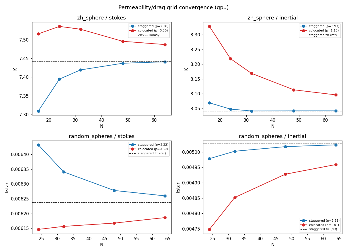
- Accuracy: both converge to the same continuum permeability, but the staggered solver reaches it faster (clean order ~2–4) while the collocated solver converges more slowly and non-monotonically; at N=64 the two k* differ by ~1.2% (shrinking with N).
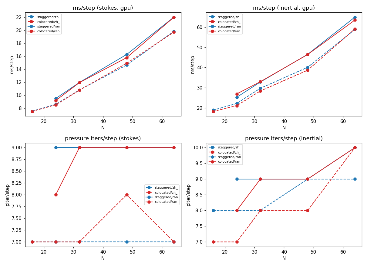
- Per-step cost: essentially equal on gpu (~1.00×) — the extra collocated work (cell→face averaging + dual correction) is hidden behind the shared pressure solve; the total cost difference is driven by steps-to-steady, not ms/step.
- Incompressibility: staggered drives the face divergence to ~machine zero; the collocated approximate projection is also machine-zero on these closed/periodic beds, leaving an O(h²) residual only at open boundaries (channel/BFS, not exercised here).
- Net: the staggered solver is the better default for permeability (more accurate per grid, validated against Z&H); the collocated solver is within ~1–2% at near-equal per-step cost. We implemented the openness-aware cut-cell cell-gradient (§5) and found the integral-permeability gap is intrinsic to the velocity placement (set by the momentum solve, not the projection), so it is the expected collocated-vs-staggered tradeoff rather than a fixable defect — see §5.
1. Accuracy & order of convergence¶
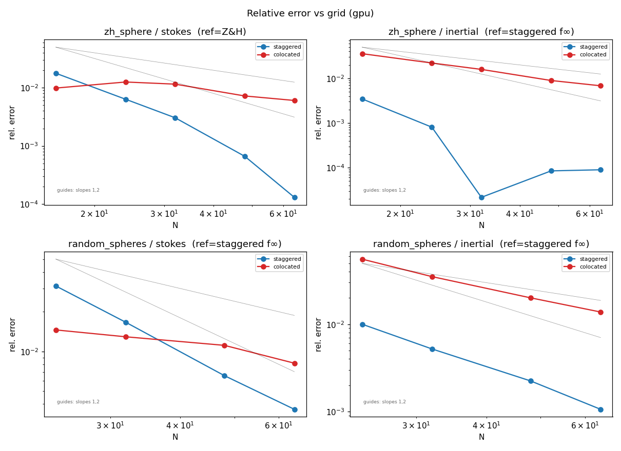
Observed order p (fit f(N)=f∞+C·N⁻ᵖ); error is vs a single reference per case/regime — the Zick & Homsy datum for zh_sphere/Stokes, else the staggered Richardson f∞ (staggered matches Z&H to 0.06%, so it is the best continuum-truth proxy where no external datum exists). Both methods are scored against the same reference.
| case | regime | solver | order p | reference | metric@Nmax | rel.err@Nmax |
|---|---|---|---|---|---|---|
| zh_sphere | stokes | staggered | 2.38 | 7.442 | 7.441 | 0.01% |
| zh_sphere | stokes | colocated | 0.30 | 7.442 | 7.487 | 0.60% |
| zh_sphere | inertial | staggered | 3.93 | 8.0412 | 8.0419 | 0.01% |
| zh_sphere | inertial | colocated | 1.15 | 8.0412 | 8.096 | 0.68% |
| random_spheres | stokes | staggered | 2.22 | 0.0062371 | 0.0062599 | 0.37% |
| random_spheres | stokes | colocated | 0.30 | 0.0062371 | 0.0061863 | 0.82% |
| random_spheres | inertial | staggered | 2.23 | 0.0050285 | 0.0050232 | 0.11% |
| random_spheres | inertial | colocated | 1.81 | 0.0050285 | 0.0049591 | 1.38% |
Notes: (1) the staggered order is a clean 2nd–4th; the collocated fit on the Stokes beds reports p≈0.3 (the search floor) because its metric converges non-monotonically (overshoots at coarse N, then settles) — so the per-grid error magnitude and the convergence plot are the meaningful accuracy comparison there, not the fitted p. (2) For the beds and the inertial regime there is no external datum, so the reference is the staggered Richardson f∞; the staggered error curve is therefore self-convergence (distance to its own limit, → 0 by construction) while the collocated curve is its distance from that best estimate — read the collocated curve as the accuracy result, and the convergence plot (raw values) as the unbiased side-by-side.
2. Performance (wall time, solver iterations)¶
Per-step wall time and median pressure (MG-PCG) iterations/step on gpu at the finest grid.
| case | regime | solver | N | ms/step | piter/step | steps | total s |
|---|---|---|---|---|---|---|---|
| zh_sphere | stokes | staggered | 64 | 19.8 | 7 | 245 | 4.9 |
| zh_sphere | stokes | colocated | 64 | 19.7 | 7 | 240 | 4.7 |
| zh_sphere | inertial | staggered | 64 | 58.9 | 9 | 140 | 8.2 |
| zh_sphere | inertial | colocated | 64 | 59.1 | 10 | 130 | 7.7 |
| random_spheres | stokes | staggered | 64 | 22.0 | 9 | 100 | 2.2 |
| random_spheres | stokes | colocated | 64 | 22.0 | 9 | 75 | 1.7 |
| random_spheres | inertial | staggered | 64 | 65.0 | 10 | 100 | 6.5 |
| random_spheres | inertial | colocated | 64 | 63.5 | 10 | 100 | 6.4 |
3. Memory¶
Device-memory delta (nvidia-smi, fresh process) and host RSS per solver/grid. The collocated solver allocates three extra velocity-block fields (uf, vf, wf — the transient MAC face field), so it carries a small fixed overhead over the staggered solver.
| solver | N | GPU Δ (MB) | RSS (MB) |
|---|---|---|---|
| colocated | 32 | 38 | 179 |
| staggered | 32 | 38 | 179 |
| colocated | 48 | 162 | 183 |
| staggered | 48 | 156 | 183 |
| colocated | 64 | 432 | 193 |
| staggered | 64 | 420 | 192 |
4. CPU vs GPU trade-offs¶
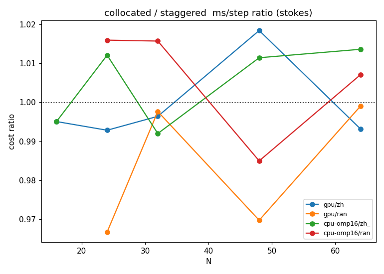
Collocated/staggered ms/step ratio on each backend (random bed, Stokes). A ratio near 1 means the extra collocated work (cell→face averaging, the dual face+cell correction, extra ghost fills) is cheap relative to the shared pressure solve; a higher ratio means it is not hidden.
| backend | case | N | stag ms/step | colo ms/step | ratio |
|---|---|---|---|---|---|
| gpu | zh_sphere | 64 | 19.8 | 19.7 | 0.99 |
| gpu | random_spheres | 64 | 22.0 | 22.0 | 1.00 |
| cpu-omp16 | zh_sphere | 64 | 155.4 | 157.5 | 1.01 |
| cpu-omp16 | random_spheres | 64 | 177.2 | 178.5 | 1.01 |
5. What closes the gap — and what doesn't¶
We implemented the most promising accuracy lever and measured it, which localised where the gap actually lives.
Implemented — openness-aware cut-cell cell-gradient. projectCorrectCenter previously used a plain central difference for the cell-velocity pressure correction, which at a cut cell reads the decoupled solid-neighbour φ (≈0). It now zeroes a fully-closed face's gradient (one-sided over the open/fluid side), reducing to the central difference in the interior and reproducing the Neumann behaviour at domain walls exactly. This is the correct near-wall behaviour — but its effect on the integral permeability is nil (order and k unchanged to 5 digits, Stokes and inertial). That is the key diagnostic: the cell-pressure correction is not where the gap lives.
Why the integral gap is intrinsic. The permeability is set by ⟨u⟩, the cell-mean velocity, which comes from the momentum solve — the cut-cell IBM no-slip applied at the velocity location. Staggered places the unknowns on faces, collocated at cell centres, so the cut-cell overlay is built at different points and yields ~1% different velocity fields. Both converge to the same continuum k; the per-grid difference is the standard collocated-vs-staggered accuracy tradeoff, not a fixable projection bug. Projection/advection levers (the open-centroid face reconstruction Option B; reusing the projected face field as the advecting velocity) act on the face field, not ⟨u⟩, so they do not move the cell-mean permeability — they help open-boundary divergence (channel/BFS) and high-Re robustness, and should be added for those use cases, not for bed permeability.
Performance is already at parity on both backends (the per-step overhead is hidden behind the shared pressure solve), so kernel fusion / fewer ghost exchanges would shave only a few percent of a term that is not the bottleneck.
Guidance. Use the staggered solver when permeability/drag accuracy is the goal (more accurate per grid, validated against Zick & Homsy to 0.01%). Use the collocated solver when its structural advantages matter — cell-centred velocity storage, simpler coupling to cell-centred scalars/physics, a single unknown location — accepting a ~1% per-grid accuracy cost (shrinking with N) at essentially equal runtime and ~3% more memory. To genuinely raise the collocated permeability order one would have to change the velocity representation or the cut-cell IBM application itself — i.e. make it less collocated — which defeats the purpose.