Immersed-boundary diffusion around two touching particles - Multiphase Reactor Modeling using PyMRM

This example demonstrates the general boundary/interface conditions of the pymrm immersed boundary method (IBM): construct_ibm_normal_derivative, construct_ibm_boundary_values and apply_ibm_interface. Two solid particles of radius $R$ touch on the centreline of a unit square filled with fluid. Steady diffusion is driven by domain boundary conditions $c=1$ (left) and $c=0$ (right), with no-flux top and bottom walls.

We solve the same geometry twice:

Impermeable particles -- in the fluid a homogeneous Neumann condition $\partial c/\partial n = 0$ is imposed at the particle surface, while the inside of the particles is held at a Dirichlet value. The two sides are completely decoupled: the immersed wall is a no-flux obstacle for the fluid.
Conjugate interface -- the particles have their own diffusion coefficient $D_\mathrm{in} \ne D_\mathrm{out}$ and the two regions are coupled through flux and value continuity at the surface.

The machinery has three layers:

construct_ibm_particles -- from the analytic Circle particles it finds the wall crossings and builds the directional ghost-cell data, with exact wall positions and outward normals (info.normals); the standard IBM object it returns feeds every step below;
construct_ibm_normal_derivative -- builds, on each side of every crossing, a one-sided formula for the outward normal derivative at the wall, $q_\mathrm{side} \approx \alpha_\mathrm{side}\, c_\Gamma^\mathrm{side} + \sum_j \gamma_j c_j$ , from generalized finite differences on same-side cells;
construct_ibm_boundary_values / apply_ibm_interface -- eliminate the unknown wall values $c_\Gamma$ from the given boundary/interface equations and fold the result into the operator matrix.

Sign convention: the derivatives are outward per side, i.e. $q_\mathrm{out}$ points out of the fluid (into the solid) and $q_\mathrm{in}$ points out of the solid, exactly as in construct_interface_matrices for grid-aligned multi-region models.

import numpy as np
from scipy.sparse.linalg import spsolve
import matplotlib.pyplot as plt
from matplotlib.patches import Circle

from pymrm import (
    construct_grad, construct_div, construct_coefficient_matrix,
    apply_ibm, apply_ibm_vector, construct_ibm_particles, Circle as Disk,
    construct_ibm_normal_derivative, construct_ibm_normal_derivative_ops,
    apply_ibm_interface, construct_ibm_boundary_values,
)

# --- Geometry and grid ---
L = 1.0                              # domain size
N = 100                              # cells per direction
R = 0.2                              # particle radius
centers = [(0.3, 0.5), (0.7, 0.5)]   # the particles touch at (0.5, 0.5)

shape = (N, N)
n = N * N
x_f = [np.linspace(0.0, L, N + 1), np.linspace(0.0, L, N + 1)]
x_c = [0.5 * (xf[:-1] + xf[1:]) for xf in x_f]
X, Y = np.meshgrid(x_c[0], x_c[1], indexing='ij')

Analytic particles, IBM data and normal-derivative operators¶

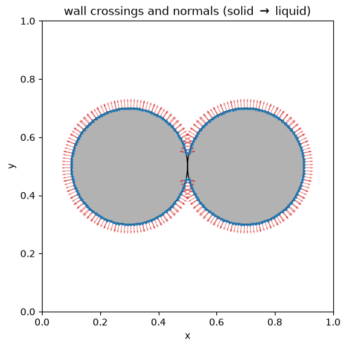
The two disks are Circle particles; construct_ibm_particles locates the wall crossings, computing each cut-face wall position and outward normal exactly from the owning circle. With contact='merge' the touching disks act as one connected solid (as a union level set would), so no artificial crossing is created between them. construct_ibm_normal_derivative then builds the one-sided normal-derivative operators used by both parts of this notebook; we pass length_scale=R so stencils never reach farther than a fraction of the particle radius, and normals=info.normals so they use the exact surface normals.

The contact point is a geometric stress test: the fluid gap between the particles pinches to zero width and the solid is connected through the contact. Because the normals come from the analytic circles they stay exact right at the contact; the GFD stencil still lowers its polynomial degree there where too few well-placed same-side cells are available (the degree_* diagnostics below), and its flood-fill connectivity filter keeps stencils from leaking through the pinch to the other side.

# The disks are described analytically.  contact='merge' keeps the union
# behaviour (touching disks act as one connected solid, as with the SDF),
# while the wall positions and normals are now exact per particle.
particles = [Disk((cx, cy), R) for cx, cy in centers]
ibm, info = construct_ibm_particles(particles, x_c, contact='merge')
sdf = info.pseudo_sdf                        # sign-correct union field
fluid = (sdf >= 0).ravel()                  # phase mask (True = liquid)
solid2d = (sdf < 0)

recon = construct_ibm_normal_derivative(ibm, sdf, x_c, length_scale=R,
                                     normals=info.normals)

print(f'wall crossings         : {ibm.n_crossings}')
for side in ('out', 'in'):
    deg = getattr(recon, f'degree_{side}')
    unres = getattr(recon, f'unresolved_{side}')
    counts = ', '.join(f'p={p}: {np.sum(deg == p)}' for p in np.unique(deg)[::-1])
    print(f'{side:>3}-side degrees used  : {counts}   (unresolved: {unres.sum()})')

fig, ax = plt.subplots(figsize=(5.5, 5.5))
ax.pcolormesh(x_f[0], x_f[1], solid2d.T, cmap='Greys', alpha=0.3, shading='flat')
ax.quiver(ibm.coords[:, 0], ibm.coords[:, 1],
          recon.normals[:, 0], recon.normals[:, 1],
          angles='xy', scale=30, width=0.002, color='tab:red', alpha=0.7)
ax.scatter(ibm.coords[:, 0], ibm.coords[:, 1], s=4, c='tab:blue', zorder=3)
for cx, cy in centers:
    ax.add_patch(Circle((cx, cy), R, fill=False, color='k', lw=1.0))
ax.set_aspect('equal')
ax.set_xlabel('x'); ax.set_ylabel('y')
ax.set_title(r'wall crossings and normals (solid $\to$ liquid)')
plt.show()

wall crossings         : 304
out-side degrees used  : p=2: 296, p=1: 8   (unresolved: 0)
 in-side degrees used  : p=2: 304   (unresolved: 0)

Bare Laplacian with the domain boundary conditions¶

We assemble the plain Laplacian $\mathsf{Lap} = \mathrm{div}(\mathrm{grad})$ once, without any diffusion coefficient, including the domain boundary conditions (Dirichlet $c=1$ left, $c=0$ right, no-flux top/bottom). The diffusion coefficient is applied afterwards as a cell-centred diagonal factor (next section), which is exactly the $-D\,\mathrm{div}(\mathrm{grad})$ form we want. The usual pymrm sign convention applies: the boundary contribution $g$ is added, so the bare-Laplacian equation reads $\mathsf{Lap}\, c + g_\mathrm{lap} = \dots$ .

bc_x = ({'a': 0, 'b': 1, 'd': 1.0}, {'a': 0, 'b': 1, 'd': 0.0})   # c=1 left, c=0 right
bc_y = ({'a': 1, 'b': 0, 'd': 0.0}, {'a': 1, 'b': 0, 'd': 0.0})   # no-flux top/bottom


def laplacian_operator():
    """Lap = div(grad) with the domain BCs; convention: Lap @ c + g_lap = source/D."""
    Lap = None
    g_lap = np.zeros(n)
    for axis, bc in enumerate((bc_x, bc_y)):
        grad, grad_bc = construct_grad(shape, x_f[axis], x_c[axis], bc=bc, axis=axis)
        div = construct_div(shape, x_f[axis], axis=axis)
        term = (div @ grad).tocsr()
        Lap = term if Lap is None else Lap + term
        g_lap += (div @ grad_bc).toarray().ravel()
    return Lap, g_lap


Lap, g_lap = laplacian_operator()

Boundary molar flows (for the overall mole balance)¶

To check the overall mole balance we need the molar flow crossing the left and right outer walls. The $x$ -derivative at the vertical grid faces is $\partial c/\partial x = \mathsf{grad}_x\, c + g_{\mathrm{grad},x}$ (the same finite-volume gradient used in the operator), and the molar flux in the $+x$ direction is $-D\,\partial c/\partial x$ . Integrating that flux over a boundary column of faces gives the molar flow (per unit depth) through that wall; both outer walls lie in the fluid, so the fluid coefficient applies there. A positive flow_left enters the domain and a positive flow_right leaves it. In steady state with no volumetric sources the two must be equal to solver precision -- the discrete finite-volume fluxes telescope, so whatever enters at the left has to leave at the right.

grad_x, grad_bc_x = construct_grad(shape, x_f[0], x_c[0], bc=bc_x, axis=0)
grad_bc_x = grad_bc_x.toarray().ravel()
dy = np.diff(x_f[1])


def boundary_molar_flows(c, D_liquid):
    """Molar flow (per unit depth) through the left and right outer boundaries."""
    dcdx = (grad_x @ c + grad_bc_x).reshape(N + 1, N)   # dc/dx at the x-faces
    flux_x = -D_liquid * dcdx                            # molar flux in +x
    flow_left = np.sum(flux_x[0, :] * dy)               # +x through x=0  (inflow)
    flow_right = np.sum(flux_x[N, :] * dy)              # +x through x=L  (outflow)
    return flow_left, flow_right

Part 1: no-flux particles (Neumann outside, Dirichlet inside)¶

On the fluid side we impose the homogeneous Neumann condition

1 \cdot q_\mathrm{out} + 0 \cdot c_\Gamma^\mathrm{out} = 0 \qquad\Longleftrightarrow\qquad \left.\frac{\partial c}{\partial n}\right|_\Gamma = 0 ,

(1)

i.e. the wall equation dictionary {'a': 1, 'b': 0, 'd': 0} (any Robin condition a*q + b*c = d works the same way). construct_ibm_boundary_values eliminates the unknown fluid-side wall value, returning it as a sparse function of the field, $c_\Gamma^\mathrm{out} = \mathsf H c + h$ . This enters the system through the wall source matrices G_out/G_in returned by apply_ibm(..., return_bc='matrix').

The solid side is completely decoupled from the fluid: there we simply prescribe a Dirichlet wall value $c_\Gamma^\mathrm{in} = c_\mathrm{solid}$ , exactly as in the plain Dirichlet IBM (a known value contributes G_in @ values to the source). Since the solid interior keeps a diffusion equation with this wall value as its only boundary condition, it relaxes to the uniform value $c_\mathrm{solid}$ -- it is only there for display; the fluid solution does not depend on it.

As with the Dirichlet IBM, any independently assembled right-hand-side contribution (here the domain-boundary vector g_bc) must pass through apply_ibm_vector so it receives the same row conditioning as the matrix.

D = 1.0          # diffusion coefficient of the liquid
c_solid = 0.5    # Dirichlet wall value seen from the inside

# -D div(grad); D is uniform here (the impermeable solid is decoupled)
L_mat = (-D * Lap).tocsr()
g_bc = -D * g_lap

# Ghost-cell folding; G_out / G_in route wall values into the cut-cell rows
A_ibm, G_out, G_in = apply_ibm(L_mat, ibm, return_bc='matrix')

# Liquid side: 1 * q_out + 0 * c_wall = 0  ->  homogeneous Neumann (no flux)
H, h = construct_ibm_boundary_values(ibm, recon,
                                     {'a': 1.0, 'b': 0.0, 'd': 0.0}, side='out')
A1 = (A_ibm + G_out @ H).tocsr()

# Solid side: known Dirichlet wall values
val_in = np.full(ibm.n_crossings, c_solid)
g1 = (apply_ibm_vector(g_bc, ibm)
      + np.asarray(G_out @ h).ravel()
      + np.asarray(G_in @ val_in).ravel())

c1 = spsolve(A1.tocsc(), -g1)          # steady state: A1 @ c + g1 = 0
c1_2d = c1.reshape(shape)

print(f'liquid min/max : {c1[fluid].min():.4f} / {c1[fluid].max():.4f}')
print(f'solid  min/max : {c1[~fluid].min():.4f} / {c1[~fluid].max():.4f}   '
      f'(should equal c_solid = {c_solid})')

liquid min/max : 0.0011 / 0.9989
solid  min/max : 0.5000 / 0.5000   (should equal c_solid = 0.5)

With impermeable particles all flux has to bend around the solid: iso-concentration lines meet the surface at right angles (zero normal derivative). The profile through the particle centreline shows the decoupling -- the solid sits at $c_\mathrm{solid}$ , independent of the neighbouring fluid values.

fig, axs = plt.subplots(1, 2, figsize=(11, 4.6))

m = axs[0].pcolormesh(x_f[0], x_f[1], c1_2d.T, shading='flat', cmap='viridis')
axs[0].contour(X, Y, np.ma.masked_array(c1_2d, mask=solid2d),
               levels=np.linspace(0.05, 0.95, 19), colors='w', linewidths=0.6)
for cx, cy in centers:
    axs[0].add_patch(Circle((cx, cy), R, fill=False, color='w', lw=1.5))
axs[0].set_aspect('equal')
axs[0].set_xlabel('x'); axs[0].set_ylabel('y')
axs[0].set_title('no-flux particles: contours bend around the solid')
fig.colorbar(m, ax=axs[0], label='c')

j_side = np.argmin(np.abs(x_c[1] - 0.25))
j_mid = np.argmin(np.abs(x_c[1] - 0.5))
axs[1].plot(x_c[0], c1_2d[:, j_side], label=f'y = {x_c[1][j_side]:.3f} (liquid)')
axs[1].plot(x_c[0], c1_2d[:, j_mid], label=f'y = {x_c[1][j_mid]:.3f} (through particles)')
axs[1].axvspan(centers[0][0] - R, centers[1][0] + R, color='grey', alpha=0.15,
               label='particle span')
axs[1].set_xlabel('x'); axs[1].set_ylabel('c')
axs[1].set_title('horizontal profiles')
axs[1].legend()
plt.tight_layout()
plt.show()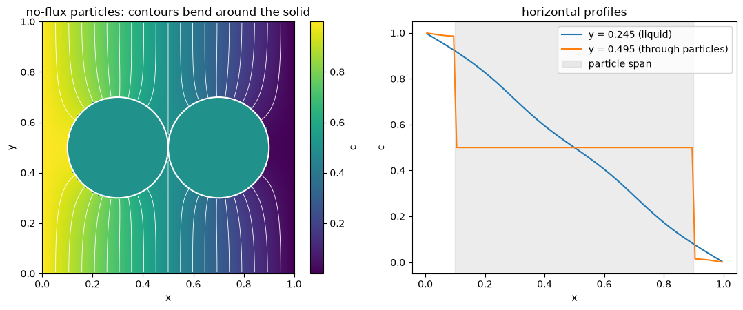

Overall mole balance. The fluid is source-free and the particle surfaces carry no flux, so every mole entering at the left must leave at the right. The empty channel (no particles) would pass $D\,\Delta c\,H/W = D = 1$ ; the impermeable particles obstruct the path and reduce the throughput below that reference.

flow_left, flow_right = boundary_molar_flows(c1, D)
print(f'left  boundary (inflow)  : {flow_left:.6f}')
print(f'right boundary (outflow) : {flow_right:.6f}')
print(f'relative imbalance       : {abs(flow_left - flow_right) / abs(flow_left):.2e}')
print(f'empty-channel reference  : {D:.6f}  '
      f'(throughput ratio {flow_left / D:.3f})')

left  boundary (inflow)  : 0.672428
right boundary (outflow) : 0.672428
relative imbalance       : 2.71e-13
empty-channel reference  : 1.000000  (throughput ratio 0.672)

Part 2: conjugate interface with different diffusion coefficients¶

Now the particles participate in the transport with their own diffusivity $D_\mathrm{in} \ne D_\mathrm{out}$ , coupled to the fluid by the conjugate interface conditions

D_\mathrm{out}\, q_\mathrm{out} + D_\mathrm{in}\, q_\mathrm{in} = 0 \qquad\text{(flux continuity)},\qquad c_\Gamma^\mathrm{out} - c_\Gamma^\mathrm{in} = 0 \qquad\text{(value continuity)} .

(2)

(Remember $q_\mathrm{out}$ and $q_\mathrm{in}$ are both outward derivatives, so flux continuity is a sum, not a difference.) In dictionary form -- identical to the ic format of construct_interface_matrices -- this is

ic = ({'a': (D_out, D_in), 'b': (0.0, 0.0), 'd': 0.0},
      {'a': (0.0, 0.0), 'b': (1.0, -1.0), 'd': 0.0})

A partition coefficient ( $c_\mathrm{out} = K\, c_\mathrm{in}$ ) or a contact resistance would only change these coefficients.

Keep the diffusion coefficient outside the Laplacian¶

Away from the interface each region has a uniform diffusion coefficient, so before the interface conditions are applied the balances are simply

\text{fluid: } -D_\mathrm{out}\nabla^2 c = 0, \qquad \text{solid: } -D_\mathrm{in}\nabla^2 c = 0 ,

(3)

i.e. the diffusion coefficient sits outside the Laplacian. We build this directly: one bare Laplacian $\mathsf{Lap} = \mathrm{div}(\mathrm{grad})$ (already assembled above) and a cell-centred field of diffusion coefficients, $D_\mathrm{out}$ in the fluid and $D_\mathrm{in}$ in the solid. construct_coefficient_matrix turns that field into a diagonal matrix $\mathsf D$ , and the operator is simply

\mathsf L = -\,\mathsf D\,\mathsf{Lap} .

(4)

Because $\mathsf D$ is diagonal it just scales each row (each cell equation) by the diffusion coefficient at that cell centre. We deliberately do not define $D$ on the cell faces through a mixture rule (harmonic or arithmetic averaging of $D_\mathrm{out}$ and $D_\mathrm{in}$ ): a face-averaged coefficient would impose its own smeared, first-order coupling across the cut cells and interfere with the sharp ghost-cell treatment. All communication between the two regions must come exclusively from the interface conditions, which apply_ibm_interface folds into the cut-cell rows.

D_out, D_in = 1.0, 5.0     # liquid / particle diffusion coefficients

# Cell-centred diffusion-coefficient field: D_out in the liquid, D_in in the solid
D_field = np.where(solid2d, D_in, D_out)          # shape (N, N)
D_mat = construct_coefficient_matrix(D_field, shape=shape)   # diagonal D matrix

# Operator -D div(grad): D outside the Laplacian, defined at cell centres
L2 = (-D_mat @ Lap).tocsr()
g2 = -(D_mat @ g_lap)

# Conjugate interface conditions: flux continuity + value continuity
ic = ({'a': (D_out, D_in), 'b': (0.0, 0.0), 'd': 0.0},
      {'a': (0.0, 0.0), 'b': (1.0, -1.0), 'd': 0.0})

A2, g_ic, (H_out, h_out, H_in, h_in) = apply_ibm_interface(
    L2, ibm, recon, ic, return_values=True)

c2 = spsolve(A2.tocsc(), apply_ibm_vector(-g2, ibm) - g_ic)
c2_2d = c2.reshape(shape)

Interface values and fluxes¶

With return_values=True we also get the elimination operators $c_\Gamma^\mathrm{side} = \mathsf H_\mathrm{side}\, c + h_\mathrm{side}$ , useful for post-processing wall concentrations and, combined with construct_ibm_normal_derivative_ops, wall fluxes. Since the elimination enforces the two interface equations exactly, the recovered values satisfy them to machine precision -- a consistency check of the assembly (the accuracy of the solution is governed by the reconstruction order, second order here).

cg_out = H_out @ c2 + h_out
cg_in = H_in @ c2 + h_in

alpha_o, N_o, alpha_i, N_i = construct_ibm_normal_derivative_ops(ibm, recon)
q_out = alpha_o * cg_out + N_o @ c2
q_in = alpha_i * cg_in + N_i @ c2

print(f'max |c_out - c_in|            : {np.abs(cg_out - cg_in).max():.2e}')
print(f'max |D_out q_out + D_in q_in| : {np.abs(D_out * q_out + D_in * q_in).max():.2e}')

max |c_out - c_in|            : 0.00e+00
max |D_out q_out + D_in q_in| : 5.12e-13

Because the particles conduct better than the fluid ( $D_\mathrm{in} = 5 D_\mathrm{out}$ ), iso-concentration lines are now attracted into the solid and refract at the surface. The centreline profile is continuous across the interfaces (value continuity) but shows a kink: flux continuity forces the slope inside the particles to be about $D_\mathrm{out}/D_\mathrm{in}$ times the outside slope.

fig, axs = plt.subplots(1, 2, figsize=(11, 4.6))

m = axs[0].pcolormesh(x_f[0], x_f[1], c2_2d.T, shading='flat', cmap='viridis')
axs[0].contour(X, Y, c2_2d, levels=np.linspace(0.05, 0.95, 19),
               colors='w', linewidths=0.6)
for cx, cy in centers:
    axs[0].add_patch(Circle((cx, cy), R, fill=False, color='w', lw=1.5))
axs[0].set_aspect('equal')
axs[0].set_xlabel('x'); axs[0].set_ylabel('y')
axs[0].set_title('conjugate particles: contours refract into the solid')
fig.colorbar(m, ax=axs[0], label='c')

j_mid = np.argmin(np.abs(x_c[1] - 0.5))
axs[1].plot(x_c[0], c2_2d[:, j_mid], label=f'y = {x_c[1][j_mid]:.3f}')
for xi in (centers[0][0] - R, 0.5, centers[1][0] + R):
    axs[1].axvline(xi, color='grey', ls=':', lw=1)
axs[1].axvspan(centers[0][0] - R, centers[1][0] + R, color='grey', alpha=0.15,
               label='particle span')
# wall concentrations of the crossings closest to the centreline
sel = np.abs(ibm.coords[:, 1] - 0.5) < 0.02
axs[1].plot(ibm.coords[sel, 0], cg_out[sel], 'o', ms=5, mfc='none',
            color='tab:red', label=r'wall values $c_\Gamma$')
axs[1].set_xlabel('x'); axs[1].set_ylabel('c')
axs[1].set_title('centreline profile: continuous value, slope kink')
axs[1].legend()
plt.tight_layout()
plt.show()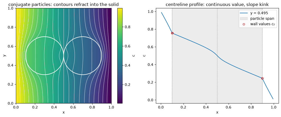

Overall mole balance. The interface conditions enforce flux continuity, so no moles accumulate at the particle surfaces; with a source-free interior the inflow again equals the outflow. Now the better-conducting particles ( $D_\mathrm{in} = 5\, D_\mathrm{out}$ ) form high-conductance bridges across the channel, so the throughput exceeds the empty-channel reference $D_\mathrm{out} = 1$ .

flow_left, flow_right = boundary_molar_flows(c2, D_out)
print(f'left  boundary (inflow)  : {flow_left:.6f}')
print(f'right boundary (outflow) : {flow_right:.6f}')
print(f'relative imbalance       : {abs(flow_left - flow_right) / abs(flow_left):.2e}')
print(f'empty-channel reference  : {D_out:.6f}  '
      f'(throughput ratio {flow_left / D_out:.3f})')

left  boundary (inflow)  : 1.553690
right boundary (outflow) : 1.553690
relative imbalance       : 2.92e-13
empty-channel reference  : 1.000000  (throughput ratio 1.554)

Summary¶

construct_ibm_normal_derivative provides one-sided normal-derivative formulas at every wall crossing; everything else in this notebook consumed them.
A single-side wall condition (Neumann/Robin in the fluid, unmodelled or pinned solid) uses construct_ibm_boundary_values together with the G_out/G_in source matrices of apply_ibm(..., return_bc='matrix').
Two-side interface conditions (conjugate transfer, partition coefficients, contact resistance) use apply_ibm_interface with the same two-equation ic dictionaries as grid-aligned construct_interface_matrices.
For piecewise-constant diffusivities, build one bare Laplacian and a cell-centred diffusion-coefficient field, then form $-\mathsf D\,\mathrm{div}(\mathrm{grad})$ with a diagonal $\mathsf D$ from construct_coefficient_matrix -- keeping $D$ outside the Laplacian, never a face-averaged $D$ -- so that the interface physics comes only from the imposed interface conditions.
The overall mole balance closes to solver precision in both cases (left inflow = right outflow): impermeable particles reduce the throughput below the empty-channel value, while better-conducting particles raise it above.