Unsteady convection + reaction 1D - Multiphase Reactor Modeling using PyMRM

Reaction: $A \rightarrow B\rightarrow C$

$\frac{\partial c_A}{\partial t} + \mathrm{div}(v \, c_A) = -k_1 \, c_A$

$\frac{\partial c_B}{\partial t} + \mathrm{div}(v \, c_B) = k_1 \, c_A - k_2 \, c_B$

$\frac{\partial c_C}{\partial t} + \mathrm{div}(v \, c_C) = k_2 \, c_B$

with boundary conditions: $c_A(0)=0.5, c_B(0)=c_C(0)=0$ , $\frac{\partial c_i(L)}{\partial x} = 0$

Imports¶

import numpy as np
from scipy.sparse import eye_array, linalg as sla
import matplotlib.pyplot as plt
from IPython.display import clear_output, display
from pymrm import construct_convflux_upwind, construct_div, NumJac, interp_cntr_to_stagg_tvd, minmod

Reaction term¶

The first-order series reaction $A \rightarrow B \rightarrow C$ ; the sum of the three rates is zero, so the total concentration is unaffected by the reaction.

def reaction(c, k_1, k_2):
    r = np.zeros_like(c)
    r[:, 0] = -k_1 * c[:, 0]
    r[:, 1] = k_1 * c[:, 0] - k_2 * c[:, 1]
    r[:, 2] = k_2 * c[:, 1]
    return r

Parameters and boundary conditions¶

Physical and numerical parameters, and the boundary dictionary in the a*dc/dn + b*c = d convention (outward normal): $c_A=0.5$ , $c_B=c_C=0$ fixed at $x=0$ , and a zero-gradient outlet at $x=L$ for every component.

# Physical parameters
L = 1
v = 0.1
k_1 = 3.0
k_2 = 1.0
t_end = 5
bc = ({'a': 0, 'b': 1, 'd': [[0.5, 0, 0]]}, {'a': 1, 'b': 0, 'd': 0})

# Numerical parameters
num_x = 1000
num_c = 3
num_time_steps = 1000
num_inner_iter = 1
output_interval = 10
dt = t_end / num_time_steps

Grid and operators¶

Uniform grid and the constant convection, divergence, and reaction Jacobian (evaluated once at $c=0$ , since the reaction is linear). The first-order upwind part of the convection is kept in the constant Jacobian; a TVD deferred correction (minmod limiter) is added explicitly in the solve loop.

c = np.zeros((num_x, num_c))
numjac = NumJac(c.shape, axes_blocks=[-1])

x_f = np.linspace(0, L, num_x + 1)
x_c = 0.5 * (x_f[:-1] + x_f[1:])

conv_mat, conv_bc = construct_convflux_upwind(c.shape, x_f, x_c, bc, v, axis=0)
div_mat = construct_div(c.shape, x_f, nu=0, axis=0)
g_const = div_mat @ conv_bc
f_react, jac_react = numjac(lambda c: reaction(c, k_1, k_2), c)
jac = eye_array(c.size, format='csc') / dt + div_mat @ conv_mat - jac_react
jac_lu = sla.splu(jac)

Solve (implicit Euler time stepping)¶

One Newton iteration per time step is enough because the reaction is linear and only the convective deferred correction is nonlinear in c. The plot is updated live every output_interval steps.

fig, ax = plt.subplots()
labels = [r'$A$', r'$B$', r'$C$']
lines = [ax.plot(x_c, c[:, j], label=labels[j])[0] for j in range(num_c)]
plt.legend()
plt.xlabel('position')
plt.ylabel('concentration')
plt.ylim(0, 0.6)
for i in range(num_time_steps):
    c_old = c.copy().reshape(-1, 1)
    for j in range(num_inner_iter):
        c_f, dc_f = interp_cntr_to_stagg_tvd(c, x_f, x_c, bc, v, minmod, axis=0)
        g_conv_deferred = div_mat @ (v * dc_f).reshape((-1, 1))
        g = g_const + jac @ c.reshape(-1, 1) - c_old / dt + g_conv_deferred
        c -= jac_lu.solve(g).reshape(c.shape)
    clear_output(wait=True)
    if i % output_interval == 0:
        for j in range(num_c):
            lines[j].set_ydata(c[:, j])
        display(fig)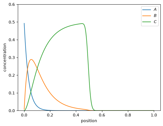

Checking the result¶

Because the reaction rates sum to zero, the total concentration $c_{tot}=c_A+c_B+c_C$ obeys plain convection with inlet value 0.5 and no reaction sink. With the front $x=vt$ still short of the outlet, the total amount of $c_{tot}$ in the domain must equal the accumulated inflow $v\,t_{end}\,c_{tot}(0)$ . This would catch a stoichiometry error in reaction, a wrong inlet value, or a convection scheme that fails to conserve the total.

c_tot = c.sum(axis=1)
dz = np.diff(x_f)
accumulated = np.sum(c_tot * dz)
expected = v * t_end * 0.5
print(f"accumulated total {accumulated:.6f}, expected v*t_end*c_in {expected:.6f}, "
      f"relative difference {(accumulated - expected) / expected:.3e}")
print("Matching to machine precision confirms the series reaction conserves the total concentration and the front has not yet left the domain.")

accumulated total 0.250000, expected v*t_end*c_in 0.250000, relative difference 5.174e-14
Matching to machine precision confirms the series reaction conserves the total concentration and the front has not yet left the domain.