Darcy flow in a 2D domain with varying permeability - Multiphase Reactor Modeling using PyMRM

\mathrm{div}\left(-\frac{k}{\mu} \mathrm{grad}(p)\right) = 0

(1)

This is 2D Darcy flow: a source-free, elliptic pressure equation for flow through a porous medium with permeability $k$ and viscosity $\mu$ . The domain contains a circular region of low permeability embedded in a higher-permeability background. The top and bottom walls are no-flux (Neumann, $\partial p/\partial n = 0$ ), and a fixed pressure drop between the left and right ends ( $p=1$ at $x=0$ , $p=0$ at $x=2L$ ) drives the flow through and around the low-permeability inclusion.

Imports¶

import math
import numpy as np
import scipy as sp
from scipy.sparse import linalg as sla
import matplotlib.pyplot as plt
from pymrm import construct_grad, construct_coefficient_matrix, construct_div, interp_stagg_to_cntr

Parameters and permeability field¶

A circular inclusion of low permeability k_int sits in a background of permeability k_ext.

# For ease of 2D plotting, and in accordance with ij indexing
# of matrices where j is the x-direction, we here associate
# x with dimension 1 and y with dimension 0

dim = 2
L = 1.0
cntr = [0.55*L, L]
R = 0.45*L
box = [L,2*L]
k_ext = 1
k_int = 0.05
mu = 1
shape_p = (100,100)

def permeability_field(x):
    x0 = x[0].reshape((-1,1))
    x1 = x[1].reshape((1,-1))
    k = k_ext + (k_int-k_ext)*(((x0-cntr[0])*(x0-cntr[0])+(x1-cntr[1])*(x1-cntr[1]))<R*R)
    return k

Grid, boundary conditions and face permeabilities¶

Axis 0 (y) has no-flux walls at both ends; axis 1 (x) has the fixed pressure drop that drives the flow.

x_f = [None] * dim
x_c = [None] * dim
for i in range(dim):
    x_f[i] = np.linspace(0,box[i], shape_p[i]+1)
    x_c[i] = 0.5*(x_f[i][1:]+x_f[i][:-1])

bc = [None]*dim
bc[0] = ({'a': 1, 'b': 0, 'd':0},)*2
bc[1] = ({'a': 0, 'b': 1, 'd':1},{'a': 0, 'b': 1, 'd':0})

# permeabilities at face positions
k_f = [None]*dim
k_f[0] = permeability_field((x_f[0], x_c[1]))
k_f[1] = permeability_field((x_c[0], x_f[1]))

Assembling the flux and divergence operators, and solving for the pressure¶

flux_mat = [None]*dim
flux_bc = [None]*dim
lapl_mat = sp.sparse.csc_array((math.prod(shape_p),math.prod(shape_p)))
lapl_bc = np.zeros((math.prod(shape_p),1))
for i in range(dim):
    grad_mat, grad_bc = construct_grad(shape_p, x_f[i], x_c[i], bc[i], axis=i)
    k_mat = construct_coefficient_matrix(k_f[i]/mu)
    flux_mat[i] = -k_mat @ grad_mat
    flux_bc[i] = - k_mat @ grad_bc
    div_mat = construct_div(shape_p, x_f[i], nu=0, axis=i)
    lapl_mat += div_mat @ flux_mat[i]
    lapl_bc += div_mat @ flux_bc[i]
lapl_lu = sla.splu(lapl_mat)
p = -lapl_lu.solve(lapl_bc).reshape(shape_p)

Cell-centered fluxes for plotting¶

flux_c = [None]*dim
for i in range(dim):
    shape_f = list(shape_p)
    shape_f[i] +=1
    flux = (flux_mat[i]@p.reshape((-1,1))+flux_bc[i]).reshape(shape_f)
    flux_c[i] = interp_stagg_to_cntr(flux, x_f[i], x_c[i], axis=i)

Pressure contour and streamlines¶

fig, ax = plt.subplots()
contour = ax.pcolormesh(x_f[1], x_f[0], p, shading='flat', cmap='viridis')
X,Y = np.meshgrid(x_c[1], x_c[0],indexing='xy')
ax.streamplot(X, Y, flux_c[1], flux_c[0], color = 'white')
ax.set_xlim(x_f[1][0], x_f[1][-1])
ax.set_ylim(x_f[0][0], x_f[0][-1])
ax.set_aspect('equal')
cbar_ax = fig.add_axes([0.92, ax.get_position().y0, 0.02, ax.get_position().y1-ax.get_position().y0])  # Adjust the parameters as needed [left, bottom, width, height]
plt.colorbar(contour, cax=cbar_ax)
plt.show()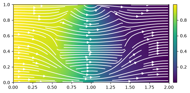

Checking the result¶

This Darcy problem is source-free and steady, so $\mathrm{div}(\mathrm{flux}) = 0$ everywhere: no reaction or accumulation term absorbs an imbalance. The net volumetric flux entering through the pressure boundary at $x=0$ must therefore equal the net flux leaving through the pressure boundary at $x=2L$ (a global mass balance). A sign error in the flux assembly, or an unconverged or wrong solve, breaks this balance.

# Global mass balance check: sum the face-normal flux (before cell-centering)
# at the two pressure (Dirichlet) faces of axis 1. We reuse the raw face-flux
# array flux_mat[1] @ p + flux_bc[1] directly, which is simpler here than
# calling compute_boundary_values since these faces already sit exactly on the
# operator's staggered grid.
shape_f1 = list(shape_p)
shape_f1[1] += 1
flux_face_x = (flux_mat[1] @ p.reshape((-1, 1)) + flux_bc[1]).reshape(shape_f1)

dy = x_f[0][1] - x_f[0][0]  # uniform grid spacing in the y-direction
flux_in = np.sum(flux_face_x[:, 0]) * dy    # entering at x = 0
flux_out = np.sum(flux_face_x[:, -1]) * dy  # leaving at x = 2L

flux_scale = 0.5 * (abs(flux_in) + abs(flux_out))
imbalance = (flux_in - flux_out) / flux_scale

print(f"Flux in  (x=0):  {flux_in: .6e}")
print(f"Flux out (x=2L): {flux_out: .6e}")
print(f"Relative imbalance: {imbalance: .3e}")
print("Imbalance at machine precision confirms mass is conserved; a large value"
      " would point to a sign error in the flux assembly or an unconverged solve.")

Flux in  (x=0):   1.757774e-01
Flux out (x=2L):  1.757774e-01
Relative imbalance:  2.430e-13
Imbalance at machine precision confirms mass is conserved; a large value would point to a sign error in the flux assembly or an unconverged solve.