Lid-driven cavity¶

This example shows that the pymrm toolbox is flexible enough to simulate incompressible Navier-Stokes flow. The governing equations are the momentum balance and the continuity (incompressibility) constraint:

\rho \left( \frac{\partial \boldsymbol{v}}{\partial t} + \boldsymbol{v} \cdot \nabla \boldsymbol{v} \right) = -\nabla p + \mu \nabla^2 \boldsymbol{v}, \qquad \nabla \cdot \boldsymbol{v} = 0

(1)

The setup is the classic lid-driven cavity: a closed square (or cubic) box with no-slip walls. The top wall (the lid) moves tangentially at a constant velocity v_top; no fluid passes through any wall. Because the box is closed, the pressure has no boundary value of its own: the pressure correction gets a zero normal gradient on every wall, and the pressure is fixed up to a constant by pinning it in one cell. The flow is solved with a fractional-step (projection) method: a momentum predictor gives a velocity field that is not yet divergence-free, then a pressure-correction Poisson equation is solved and used to project the velocity back onto the divergence-free subspace.

The setup is quite involved because of the staggered mesh: pressure lives at cell centers, and each velocity component lives on its own staggered grid, shifted by half a cell in its own direction. A surprising finding is that in almost all cases the direct sparse solver is faster (or as fast) as ilu + bicgstab.

Imports¶

import numpy as np
import scipy as sp
from scipy.sparse import linalg as sla
from scipy.sparse import eye_array
import matplotlib.pyplot as plt
from IPython.display import clear_output
from pymrm import interp_stagg_to_cntr, interp_cntr_to_stagg, interp_cntr_to_stagg_tvd
from pymrm import construct_grad, construct_div, minmod

Physical and numerical parameters¶

# Physical Parameters
dim = 2
rho = 1
mu = 1
p_ref = 0  # pressure in the reference cell (the pressure is fixed up to a constant)
v_top = 100  # Reynolds number rho * v_top * L / mu = 100
box = [1.0] * dim

# Numerical Parameters
shape_p = [50] * dim
Co = 0.5
dt = Co*(box[0]/v_top)/shape_p[0]
max_time_steps = 5000
steady_tol = 1e-8  # stop when the largest velocity change per step is below steady_tol * v_top
plot_every = 500

Grid setup and boundary conditions¶

Pressure lives on a cell-centered grid; each velocity component v[i] lives on a grid staggered by half a cell along its own axis i (a face-centered grid in that direction, cell-centered in the others). Boundary conditions use the OUTWARD normal, so the same {'a', 'b', 'd'} dictionary means opposite gradients at the two ends of an axis. The lid velocity is imposed by setting bc_v[0][-1][1]['d'] = v_top: the x-velocity (component 0), along the last axis (dim - 1, pointing up), at its upper end (index 1). All other velocity conditions are no-slip, and the normal velocity on every wall is zero by construction: each velocity component is stored on the interior faces of its own axis only, and the wall values are padded with zeros. The pressure gets a zero normal gradient on all walls.

x_cntr_c  = [None] * dim  # cell-centered positions
x_cntr_f  = [None] * dim  # cell face positions
x_stagg_c = [None] * dim  # staggered positions for velocities
x_stagg_f = [None] * dim  # face-positions corresponding to staggered cells
shape_v   = [None] * dim  # sizes velocity ndarrays
bc_v      = [None] * dim  # velocity bc
v         = [None] * dim
v_old     = [None] * dim
v_cntr    = [None] * dim
bc_p      = [None] * dim

for i in range(dim):
    shape_v[i] = shape_p.copy()
    x_cntr_f[i]  = np.linspace(0, box[i], shape_p[i]+1)
    x_cntr_c[i]  = 0.5*(x_cntr_f[i][:-1]+x_cntr_f[i][1:])
    x_stagg_c[i] = x_cntr_f[i][1:-1]
    x_stagg_f[i] = np.concatenate((x_cntr_f[i][0:1], x_cntr_c[i][1:-1], x_cntr_f[i][-1:]), axis=0)
    bc_p[i] = ({'a': 1, 'b': 0, 'd': 0},)*2
    bc_v[i] = [None] * dim
    for j in range(dim):
        shape_v[i][j] = shape_p[j]
        bc_v[i][j] = ({'a': 0, 'b': 1, 'd': 0}, {'a': 0, 'b': 1, 'd': 0})
    shape_v[i][i] -= 1
bc_v[0][-1][1]['d'] = v_top  # the lid moves in the x direction

Operators: gradient, divergence, Laplacian, Jacobians, preconditioners¶

For pressure and for each velocity component, the gradient, divergence and Laplacian operators are assembled once per axis and kept as constant sparse matrices. The momentum Jacobian jac_mat_v[i] = (rho/dt) * eye - mu * lapl_mat_v[i] is the implicit-Euler operator for the momentum predictor; an ILU factorization of it is built once and reused as a preconditioner inside the time loop; the pressure Laplacian gets a direct LU factorization. With zero-gradient conditions on all walls the pressure Laplacian is singular (a constant can be added to the pressure); replacing the equation of one reference cell by dp = 0 removes the constant. The other equations still enforce continuity in that cell, because the divergences of a closed box sum to zero.

grad_mat_v    = [None] * dim
grad_bc_v = [None] * dim
div_mat_v     = [None] * dim
lapl_mat_v    = [None] * dim
lapl_bc_v = [None] * dim
jac_mat_v     = [None] * dim
jac_pc_v  = [None] * dim
g_v       = [None] * dim
grad_mat_p    = [None] * dim
grad_bc_p = [None] * dim
div_mat_p     = [None] * dim
p = p_ref*np.ones(shape_p)
lapl_mat_p    = sp.sparse.csc_array((p.size, p.size))
lapl_bc_p = sp.sparse.csc_array((p.size, 1))

for i in range(dim):
    grad_mat_p[i], grad_bc_p[i] = construct_grad(shape_p, x_cntr_f[i], x_cntr_c[i], bc_p[i], axis=i)
    div_mat_p[i] = construct_div(shape_p, x_cntr_f[i], nu=0, axis=i)
    lapl_mat_p = lapl_mat_p + div_mat_p[i] @ grad_mat_p[i]
    lapl_bc_p = lapl_bc_p + div_mat_p[i] @ grad_bc_p[i]

    grad_mat_v[i]    = [None] * dim
    grad_bc_v[i] = [None] * dim
    div_mat_v[i]     = [None] * dim
    v[i] = np.zeros(shape_v[i])
    lapl_mat_v[i] = sp.sparse.csc_array((v[i].size, v[i].size))
    lapl_bc_v[i] = sp.sparse.csc_array((v[i].size, 1))
    for j in range(dim):
        if (i == j):
            grad_mat_v[i][j], grad_bc_v[i][j] = construct_grad(shape_v[i], x_stagg_f[j], x_stagg_c[j], bc_v[i][j], axis=j)
            div_mat_v[i][j] = construct_div(shape_v[i], x_stagg_f[j], nu=0, axis=j)
        else:
            grad_mat_v[i][j], grad_bc_v[i][j] = construct_grad(shape_v[i], x_cntr_f[j], x_cntr_c[j], bc_v[i][j], axis=j)
            div_mat_v[i][j] = construct_div(shape_v[i], x_cntr_f[j], nu=0, axis=j)
        lapl_mat_v[i] = lapl_mat_v[i] + div_mat_v[i][j] @ grad_mat_v[i][j]
        lapl_bc_v[i] = lapl_bc_v[i] + div_mat_v[i][j] @ grad_bc_v[i][j]
    jac_mat_v[i] = (rho/dt) * eye_array(v[i].size, format='csc') - mu * lapl_mat_v[i]
    jac_ilu_v = sla.spilu(jac_mat_v[i])
    jac_pc_v[i] = sla.LinearOperator(jac_ilu_v.shape, lambda x: jac_ilu_v.solve(x))
# pin the pressure correction in the reference cell (index 0, bottom-left corner)
i_ref = 0
lapl_mat_p = lapl_mat_p.tolil()
lapl_mat_p[i_ref, :] = 0
lapl_mat_p[i_ref, i_ref] = 1
lapl_mat_p = lapl_mat_p.tocsc()
lapl_lu_p = sla.splu(lapl_mat_p)

Time marching: projection method¶

The time loop marches to steady state: it stops when the largest velocity change in one step drops below steady_tol * v_top, and plots the pressure field and streamlines every plot_every steps. Each time step performs a fractional-step (projection) update:

Momentum predictor: assemble the TVD-limited (minmod) convective flux and the pressure gradient from the previous step, then solve the implicit momentum equation for each velocity component with bicgstab, preconditioned by the ILU factorization built above.
Pressure correction: solve a Poisson equation for the pressure correction dp from the divergence of the predicted velocity, using the direct sparse LU solve lapl_lu_p.solve(...).
Velocity correction: project the velocity back onto the divergence-free subspace using the pressure-correction gradient.

X, Y = np.meshgrid(x_cntr_c[0], x_cntr_c[1])

for k in range(max_time_steps):
    v_prev = [v_i.copy() for v_i in v]
    div_v = np.zeros((p.size, 1))
    for i in range(dim):
        v_old[i] = v[i].copy()
        g_conv = np.zeros((v[i].size, 1))
        for j in range(dim):
            if (j == i):
                v_f = interp_cntr_to_stagg(v[i], x_stagg_f[i], x_stagg_c[i], axis=i)
                vi_f, dvi_f = interp_cntr_to_stagg_tvd(v[i], x_stagg_f[i], x_stagg_c[i], bc_v[i][j], v_f, minmod, axis=j)
                conv_flux = rho*vi_f*vi_f
            else:
                v_f = interp_stagg_to_cntr(v[j], x_cntr_c[i], x_stagg_c[i], axis=i)
                shape_v_f_bnd = list(v_f.shape)
                shape_v_f_bnd[j] = 1
                v_f = np.concatenate((np.zeros(shape_v_f_bnd), v_f, np.zeros(shape_v_f_bnd)), axis=j)
                vi_f, dvi_f = interp_cntr_to_stagg_tvd(v[i], x_cntr_f[j], x_cntr_c[j], bc_v[i][j], v_f, minmod, axis=j)
                conv_flux = rho*v_f*vi_f
            g_conv = g_conv + div_mat_v[i][j] @ conv_flux.reshape(-1, 1)
        shape_p_f = shape_p.copy()
        shape_p_f[i] = shape_p[i]+1
        grad_p = (grad_mat_p[i] @ p.reshape(-1, 1) + grad_bc_p[i]).reshape(shape_p_f)
        idx = [slice(None)] * dim
        idx[i] = slice(1, shape_p_f[i]-1)
        g_grad_p = grad_p[tuple(idx)].reshape(-1, 1)
        g_v[i] = jac_mat_v[i] @ v[i].reshape(-1, 1) - (rho/dt)*v_old[i].reshape(-1, 1) + g_conv + g_grad_p - mu*lapl_bc_v[i]
        dv, exit_code = sla.bicgstab(jac_mat_v[i], g_v[i], M=jac_pc_v[i])
        #jac_lu = sla.splu(jac_mat_v[i])
        #dv = jac_lu.solve(g_v[i])
        v[i] -= dv.reshape(shape_v[i])

        shape_v_bnd = list(v[i].shape)
        shape_v_bnd[i] = 1
        v_incl_wall = np.concatenate((np.zeros(shape_v_bnd), v[i], np.zeros(shape_v_bnd)), axis=i)
        v_cntr[i] = interp_stagg_to_cntr(v_incl_wall, x_cntr_f[i], x_cntr_c[i], axis=i)
        div_v += div_mat_p[i] @ v_incl_wall.reshape(-1, 1)

    rhs_p = (rho/dt)*div_v
    rhs_p[i_ref] = 0  # dp = 0 in the reference cell
    dp = lapl_lu_p.solve(rhs_p)
    p += dp.reshape(shape_p)
    for i in range(dim):
        shape_p_f = shape_p.copy()
        shape_p_f[i] = shape_p[i]+1
        grad_dp = (grad_mat_p[i] @ dp.reshape(-1, 1)).reshape(shape_p_f)
        idx = [slice(None)] * dim
        idx[i] = slice(1, shape_p_f[i]-1)
        v[i] -= (dt/rho) * grad_dp[tuple(idx)]
        shape_v_bnd = list(v[i].shape)
        shape_v_bnd[i] = 1
        v_incl_wall = np.concatenate((np.zeros(shape_v_bnd), v[i], np.zeros(shape_v_bnd)), axis=i)
        v_cntr[i] = interp_stagg_to_cntr(v_incl_wall, x_cntr_f[i], x_cntr_c[i], axis=i)
    change = max(np.max(np.abs(v[i] - v_prev[i])) for i in range(dim)) / v_top
    steady = change < steady_tol
    if k % plot_every != 0 and not steady:
        continue
    clear_output(wait=True)
    plt.figure()
    contour = plt.pcolormesh(x_cntr_f[0], x_cntr_f[1], p.T, shading='flat', cmap='viridis')
    plt.streamplot(X, Y, v_cntr[0].T, v_cntr[1].T, color='white')
    plt.xticks([])
    plt.yticks([])
    plt.colorbar(contour, label='Pressure')
    plt.title(f"Time step {k}, t = {(k + 1) * dt:.3f}")
    plt.show()
    if steady:
        print(f"steady state after {k + 1} steps, t = {(k + 1) * dt:.3f}")
        break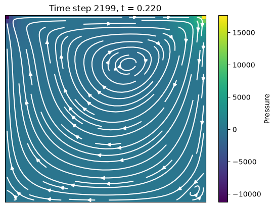

steady state after 2200 steps, t = 0.220

Checking the result¶

The projection step exists to make the velocity field satisfy the discrete continuity equation. Recompute the divergence of the final velocity in every pressure cell, with the zero wall values padded exactly as in the time loop, and compare it with the velocity scale v_top / box[0]. A relative value near round-off confirms the projection; a large value in a few cells points at an inconsistent boundary condition for the pressure correction (for example a fixed pressure on a wall through which no fluid can flow).

div_v_final = np.zeros((p.size, 1))
for i in range(dim):
    shape_v_bnd = list(v[i].shape)
    shape_v_bnd[i] = 1
    v_incl_wall = np.concatenate((np.zeros(shape_v_bnd), v[i], np.zeros(shape_v_bnd)), axis=i)
    div_v_final += div_mat_p[i] @ v_incl_wall.reshape(-1, 1)

div_scale = v_top / box[0]
print(f"max |div v| / (v_top / L) = {np.max(np.abs(div_v_final)) / div_scale:.2e}")
print(f"pressure in the reference cell: {p.ravel()[i_ref]:.3g} (p_ref = {p_ref})")

max |div v| / (v_top / L) = 1.66e-14
pressure in the reference cell: 2.23e-12 (p_ref = 0)

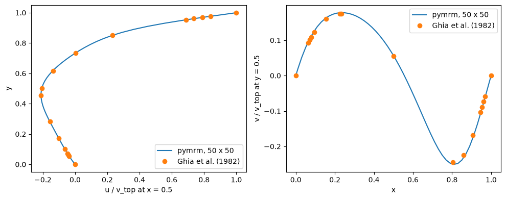
Comparison with Ghia, Ghia and Shin (1982)¶

The standard benchmark for this flow is the table of Ghia, Ghia and Shin (J. Comput. Phys. 48, 387-411, 1982): the horizontal velocity along the vertical centreline and the vertical velocity along the horizontal centreline, at steady state, computed on a fine multigrid solution. At Re = 100 the values below are from their Tables I and II. (Two neighbouring entries of the vertical-velocity table, at x = 0.9531 and x = 0.9453, appear in swapped order in some reproductions; they are given here in the order that makes the profile monotone.)

Both components are read on the staggered faces that lie exactly on the centrelines, padded with the wall values, and interpolated to the tabulated positions. The differences are scaled by the lid velocity; on this 50 x 50 grid they stay below 0.01.

Refining the grid shows that this remaining difference comes from the table, not from the model. On 100 x 100 and 200 x 200 grids the profiles change by at most 0.0028 and then 0.0006, converging at second order (observed orders 1.9 to 2.3 at the velocity extrema) to values that differ from the table by up to 0.009. For example, the minimum of the horizontal velocity at y = 0.4531 goes from -0.2112 (50 cells) to -0.2133 (100) and -0.2138 (200), with an extrapolated value of -0.2140, against -0.2109 in the table. Ghia’s values come from a 129 x 129 grid and underestimate the velocity extrema by 1 to 3 %. A sign or index error in the operators, or a flow that is not yet steady, shows up as far larger differences.

# Ghia et al. (1982), Re = 100
ghia_y = np.array([1.0, 0.9766, 0.9688, 0.9609, 0.9531, 0.8516, 0.7344, 0.6172, 0.5,
                   0.4531, 0.2813, 0.1719, 0.1016, 0.0703, 0.0625, 0.0547, 0.0])
ghia_u = np.array([1.0, 0.84123, 0.78871, 0.73722, 0.68717, 0.23151, 0.00332, -0.13641, -0.20581,
                   -0.21090, -0.15662, -0.10150, -0.06434, -0.04775, -0.04192, -0.03717, 0.0])
ghia_x = np.array([1.0, 0.9688, 0.9609, 0.9531, 0.9453, 0.9063, 0.8594, 0.8047, 0.5,
                   0.2344, 0.2266, 0.1563, 0.0938, 0.0781, 0.0703, 0.0625, 0.0])
ghia_v = np.array([0.0, -0.05906, -0.07391, -0.08864, -0.10313, -0.16914, -0.22445, -0.24533, 0.05454,
                   0.17527, 0.17507, 0.16077, 0.12317, 0.10890, 0.10091, 0.09233, 0.0])

# x-velocity on the face x = 0.5, from the bottom wall (0) to the lid (v_top)
i_mid = shape_p[0] // 2 - 1  # interior face index of x = 0.5
y_line = np.concatenate(([0.0], x_cntr_c[1], [box[1]]))
u_line = np.concatenate(([0.0], v[0][i_mid, :], [v_top])) / v_top
# y-velocity on the face y = 0.5, zero at the side walls
j_mid = shape_p[1] // 2 - 1
x_line = np.concatenate(([0.0], x_cntr_c[0], [box[0]]))
w_line = np.concatenate(([0.0], v[1][:, j_mid], [0.0])) / v_top

du = np.interp(ghia_y, y_line, u_line) - ghia_u
dv = np.interp(ghia_x, x_line, w_line) - ghia_v
print(f"centreline faces at x = {x_stagg_c[0][i_mid]:.3f} and y = {x_stagg_c[1][j_mid]:.3f}")
print(f"max |u - u_Ghia| / v_top = {np.max(np.abs(du)):.4f}")
print(f"max |v - v_Ghia| / v_top = {np.max(np.abs(dv)):.4f}")

fig, (ax_u, ax_v) = plt.subplots(1, 2, figsize=(10, 4))
ax_u.plot(u_line, y_line, '-', label=f'pymrm, {shape_p[0]} x {shape_p[1]}')
ax_u.plot(ghia_u, ghia_y, 'o', label='Ghia et al. (1982)')
ax_u.set_xlabel('u / v_top at x = 0.5')
ax_u.set_ylabel('y')
ax_u.legend()
ax_v.plot(x_line, w_line, '-', label=f'pymrm, {shape_p[0]} x {shape_p[1]}')
ax_v.plot(ghia_x, ghia_v, 'o', label='Ghia et al. (1982)')
ax_v.set_xlabel('x')
ax_v.set_ylabel('v / v_top at y = 0.5')
ax_v.legend()
plt.tight_layout()
plt.show()

centreline faces at x = 0.500 and y = 0.500
max |u - u_Ghia| / v_top = 0.0033
max |v - v_Ghia| / v_top = 0.0069