Membrane Model (Sievert’s Law Coupling) - Multiphase Reactor Modeling using PyMRM

A 2D membrane model with a shell-in-tube geometry: counter-current plug flow with radial diffusion. A membrane separates the inner retentate side from the outer annular permeate side, and a substance permeates from one side to the other through the membrane.

This notebook is the Sievert’s-law variant of the plain membrane model (membrane_module_2D.ipynb): instead of a driving force linear in concentration, the membrane flux follows the square root of partial pressure, which makes the interface condition nonlinear and requires a Newton loop.

On both sides the governing equation is:

\frac{\partial c}{\partial t} + \mathrm{div}_z (v \, c) - \mathrm{div}_r (D \, \mathrm{div}_r(c)) = 0

(1)

At the retentate and permeate sides of the membrane, Sievert’s law gives the interface conditions:

D \frac{\partial c_\mathrm{ret}}{\partial n} = P \, (\sqrt{p_\mathrm{perm}} - \sqrt{p_\mathrm{ret}}), \qquad \frac{R_\mathrm{perm}}{R_\mathrm{ret}} D \frac{\partial c_\mathrm{perm}}{\partial n} = P \, (\sqrt{p_\mathrm{ret}} - \sqrt{p_\mathrm{perm}})

(2)

with the partial pressure taken from the ideal-gas relation $p = R_g T c$ . Here $n$ is the outward normal of each subdomain. pymrm boundary conditions always use the outward normal (pitfall P1): the membrane interface is the upper radial boundary of the retentate domain, so there $\partial/\partial n = \partial/\partial r$ , while it is the lower radial boundary of the permeate domain, so there $\partial/\partial n = -\partial/\partial r$ . The two conditions above look alike but therefore impose opposite-signed fluxes when written in terms of $r$ .

The notebook is organised as parameter and grid setup, a mass-balance check, and the implicit Newton-coupled solve, ending with a check of the boundary conditions actually imposed at the interface.

import numpy as np
from matplotlib import pyplot as plt
import scipy.sparse.linalg as sla
from pymrm import construct_grad, construct_div, update_array_indices, construct_convflux_upwind, construct_interface_matrices, NumJac

L = 0.2
D = 1e-4
P = 5e-6
Rg = 8.314
T = 500
c_in = 1e4/(Rg*T)
v_ret = 1e-2
v_perm = 5e-2
R_ret = 5e-3
R_perm = R_ret + 5e-4
R_out = 7e-3

num_z = 100
num_r_perm = 10
num_r_ret = 10
num_iter = 20
tol = 1e-7

dz = L/num_z
z_f = np.linspace(0, L, num_z+1)
z_c = 0.5*(z_f[1:] + z_f[:-1])
r_f_ret = np.linspace(0, R_ret, num_r_ret+1)
r_c_ret = 0.5*(r_f_ret[1:] + r_f_ret[:-1])
r_f_perm = np.linspace(R_perm, R_out, num_r_perm+1)
r_c_perm = 0.5*(r_f_perm[1:] + r_f_perm[:-1])

bc_neumann = {'a': 1, 'b': 0, 'd': 0}
bc_dirichlet = {'a': 0, 'b': 1, 'd': 1}

shape_ret = (num_z, num_r_ret)
shape_perm = (num_z, num_r_perm)
shape_d = (num_z, 1)

div_ret_mat_z = construct_div(shape_ret, z_f, axis=0, nu=0)
div_ret_mat_r = construct_div(shape_ret, r_f_ret, axis=1, nu=1)
div_perm_mat_z = construct_div(shape_perm, z_f, axis=0, nu=0)
div_perm_mat_r = construct_div(shape_perm, r_f_perm, axis=1, nu=1)

conv_ret_mat, conv_ret_bc = construct_convflux_upwind(shape_ret, z_f, z_c, (bc_dirichlet, bc_neumann), v_ret, axis = 0)
conv_ret_bc *= c_in
conv_perm_mat, conv_perm_bc = construct_convflux_upwind(shape_perm, z_f, z_c, (bc_neumann, bc_dirichlet), -v_perm, axis = 0)
conv_perm_bc *= 0.0

from pymrm import compute_boundary_values

def print_balances():
    c_in_ret, _, c_out_ret, _  = compute_boundary_values(c_ret, z_f, z_c, ({'a':0, 'b': 1, 'd':c_in}, bc_neumann), axis=0)
    c_out_perm, _, c_in_perm, _  = compute_boundary_values(c_perm, z_f, z_c, (bc_neumann, {'a':0, 'b': 1, 'd':0}), axis=0)
    dA_r_ret = np.pi*(r_f_ret[1:]**2 - r_f_ret[:-1]**2).reshape((1,-1))
    dA_r_perm = np.pi*(r_f_perm[1:]**2 - r_f_perm[:-1]**2).reshape((1,-1))

    _, _, _, grad_mem_ret  = compute_boundary_values(c_ret, r_f_ret, r_c_ret, (bc_neumann, {'a':0, 'b': 1, 'd':c_b_ret}), axis=1)
    _ , grad_mem_perm, _, _  = compute_boundary_values(c_perm, r_f_perm, r_c_perm, ({'a':0, 'b': 1, 'd':c_b_perm}, bc_neumann), axis=1)
    dA_z_ret = 2*np.pi*R_ret*(z_f[1:] - z_f[:-1]).reshape((-1,1))
    dA_z_perm = 2*np.pi*R_perm*(z_f[1:] - z_f[:-1]).reshape((-1,1))

    flow_in_ret = v_ret*np.sum(c_in_ret*dA_r_ret, axis=1).reshape(())
    flow_out_ret = v_ret*np.sum(c_out_ret*dA_r_ret, axis=1).reshape(())
    flow_in_perm = v_perm*np.sum(c_in_perm*dA_r_perm, axis=1).reshape(())
    flow_out_perm = v_perm*np.sum(c_out_perm*dA_r_perm, axis=1).reshape(())
    flow_mem_ret = -D*np.sum(grad_mem_ret*dA_z_ret, axis=0).reshape(())
    flow_mem_perm = -D*np.sum(grad_mem_perm*dA_z_perm, axis=0).reshape(())

    print(f"retentate side: inlet molar flow = {flow_in_ret:.5e}, membrane molar flow out = {flow_mem_ret:.5e}, outlet molar flow = {flow_out_ret:.5e}")
    print(f"retentate balance: {flow_in_ret - flow_mem_ret - flow_out_ret:.5e}")
    print(f"permeate side:  inlet molar flow = {flow_in_perm:.5e}, membrane molar flow in  = {flow_mem_perm:.5e}, outlet molar flow = {flow_out_perm:.5e}")
    print(f"permeate balance: {flow_in_perm + flow_mem_perm - flow_out_perm:.5e}")
    print(f"overall balance: {flow_in_ret + flow_in_perm - flow_out_ret - flow_out_perm:.5e}")

Implicit Coupling¶

Both sides are solved as one coupled system, as in the implicit-coupling section of the plain membrane model, but here the membrane flux follows Sievert’s law, $N = P(\sqrt{p_\mathrm{perm}} - \sqrt{p_\mathrm{ret}})$ , instead of a driving force linear in concentration. Because Sievert’s law is nonlinear in the interface concentration, the interface conditions are linearized and updated in a Newton loop instead of being assembled once.

Interface Matrices and Jacobian Assembly¶

Build the constant part of the coupled Jacobian (retentate and permeate transport, without the membrane coupling), then the Neumann-type interface matrices that turn an interface flux into an interface (Dirichlet) value. These are reused every Newton iteration to linearize Sievert’s law about the current interface concentrations.

c_all = np.zeros((num_z, num_r_ret + num_r_perm))
c_ret = c_all[:, :num_r_ret]
c_perm = c_all[:, num_r_ret:]
c_vect = c_all.reshape((-1,1))

shape_ret = c_ret.shape
shape_perm = c_perm.shape
shape_d = (num_z, 1)

grad_ret_mat, _, grad_ret_bc = construct_grad(shape_ret, r_f_ret, r_c_ret, bc = (bc_neumann, bc_dirichlet), axis = 1, shapes_d = (None, shape_d))
jac_ret_mat = div_ret_mat_z @ conv_ret_mat - D*div_ret_mat_r @ grad_ret_mat
g_ret_bc  = div_ret_mat_z @ conv_ret_bc
jac_ret_dirichlet_bc  = -D*div_ret_mat_r @ grad_ret_bc
jac_ret_dirichlet_bc = update_array_indices(jac_ret_dirichlet_bc, (shape_ret, None), (c_all.shape, None), offset=None)
jac_ret_mat = update_array_indices(jac_ret_mat, shape_ret, c_all.shape, offset=None)
g_ret_bc = update_array_indices(g_ret_bc, (shape_ret, None), (c_all.shape, None), offset=None)

grad_perm_mat, grad_perm_bc, _ = construct_grad(shape_perm, r_f_perm, r_c_perm, bc=(bc_dirichlet, bc_neumann), axis = 1, shapes_d = (shape_d, None))
jac_perm_mat = div_perm_mat_z @ conv_perm_mat - D*div_perm_mat_r @ grad_perm_mat
g_perm_bc  = div_perm_mat_z @ conv_perm_bc*0
jac_perm_dirichlet_bc  = -D*div_perm_mat_r @ grad_perm_bc
jac_perm_dirichlet_bc = update_array_indices(jac_perm_dirichlet_bc, (shape_perm, None), (c_all.shape, None), offset=((0,shape_ret[1]),None))
jac_perm_mat = update_array_indices(jac_perm_mat, shape_perm, c_all.shape, offset=(0,shape_ret[1]))
g_perm_bc = update_array_indices(g_perm_bc, (shape_perm, None), (c_all.shape, None), offset=((0,shape_ret[1]),None))

jac_decoupled = jac_ret_mat + jac_perm_mat

# interface conditions:
ic_1_neumann = {'a':(D,0), 'd':P}
ic_2_neumann = {'a':(0,R_perm/R_ret*D), 'd':-P}
interf_mat_ret_neumann, interf_mat_ret_neumann_bc_0, interf_mat_ret_neumann_bc_1, interf_mat_perm_neumann, interf_mat_perm_neumann_bc_0, interf_mat_perm_neumann_bc_1 = construct_interface_matrices((shape_ret, shape_perm), (r_f_ret, r_f_perm), ic=(ic_1_neumann, ic_2_neumann), axis=1, shapes_d=(shape_d, shape_d))
jac_ret_ic_neumann = jac_ret_dirichlet_bc @ interf_mat_ret_neumann
jac_perm_ic_neumann = jac_perm_dirichlet_bc @ interf_mat_perm_neumann
interf_mat_ret_neumann_bc = interf_mat_ret_neumann_bc_0 + interf_mat_ret_neumann_bc_1
jac_ret_bc_neumann = jac_ret_dirichlet_bc @ interf_mat_ret_neumann_bc
interf_mat_perm_neumann_bc = interf_mat_perm_neumann_bc_0 + interf_mat_perm_neumann_bc_1
jac_perm_bc_neumann = jac_perm_dirichlet_bc @ interf_mat_perm_neumann_bc
jac_g = jac_decoupled + jac_ret_ic_neumann + jac_perm_ic_neumann
jac_g_ic = jac_ret_bc_neumann + jac_perm_bc_neumann

def driving_force(c_b, eps=0.1):
    return Rg*T*c_b / np.sqrt(np.abs(Rg*T*c_b) + eps)

numjac = NumJac(shape=(*shape_d, 1))

Newton Iteration for the Sievert Coupling¶

At each iteration, the Sievert driving force $P(\sqrt{p_\mathrm{perm}} - \sqrt{p_\mathrm{ret}})$ is linearized about the current interface concentrations (driving_force, regularized near $c_b = 0$ to keep its derivative finite), the interface matrices are rebuilt with the resulting local slope, and the coupled linear system is solved for the Newton step and the updated interface concentrations. The loop stops early once the residual norm drops below tol.

c_b_ret = np.zeros(shape_d)
c_b_perm = np.zeros(shape_d)
c_b_ret_vect = c_b_ret.reshape((-1,1))
c_b_perm_vect = c_b_perm.reshape((-1,1))

# Newton-Raphson:
norm = 1.0
for i in range(num_iter):
    g_d_ret, jac_b_ret = numjac(driving_force, c_b_ret)
    g_d_perm, jac_b_perm = numjac(driving_force, c_b_perm)
    g = g_ret_bc + g_perm_bc + jac_g @ c_vect + jac_g_ic @ (g_d_perm - g_d_ret).reshape((-1,1))
    norm = np.linalg.norm(g)
    b_vect_ret = jac_b_ret.data.reshape(shape_d)
    b_vect_perm = jac_b_perm.data.reshape(shape_d)
    ic_1 = {'a':(D,0), 'b':(P*b_vect_ret,-P*b_vect_perm)}
    ic_2 = {'a':(0,R_perm/R_ret*D), 'b':(-P*b_vect_ret,P*b_vect_perm)}
    interf_mat_ret, _, interf_mat_perm, _ = construct_interface_matrices((shape_ret, shape_perm), (r_f_ret, r_f_perm), ic=(ic_1, ic_2), axis=1)
    jac_ret_ic = jac_ret_dirichlet_bc @ interf_mat_ret
    jac_perm_ic = jac_perm_dirichlet_bc @ interf_mat_perm
    jac_coupled = jac_decoupled + jac_ret_ic + jac_perm_ic

    dc = -sla.spsolve(jac_coupled, g).reshape((-1,1))
    c_vect[:] = c_vect + dc

    c_b_ret_vect[:] = c_b_ret_vect + interf_mat_ret @ dc
    c_b_perm_vect[:] = c_b_perm_vect + interf_mat_perm @ dc
    d = (driving_force(c_b_perm) - driving_force(c_b_ret)).reshape((-1,1))
    c_b_ret_vect[:] = interf_mat_ret_neumann @ c_vect + interf_mat_ret_neumann_bc @ d  # here is an issue
    c_b_perm_vect[:] = interf_mat_perm_neumann @ c_vect + interf_mat_perm_neumann_bc @ d
    if norm < tol:
        break

Plot and Balance Check¶

Plot the retentate and permeate concentration fields and confirm mass is conserved with print_balances().

plt.pcolormesh(z_f, r_f_ret, c_ret.transpose(), shading='flat', cmap='viridis', vmin=0, vmax=c_in)
plt.pcolormesh(z_f, r_f_perm, c_perm.transpose(), shading='flat', cmap='viridis', vmin=0, vmax=c_in)
plt.colorbar()
plt.show()

print_balances()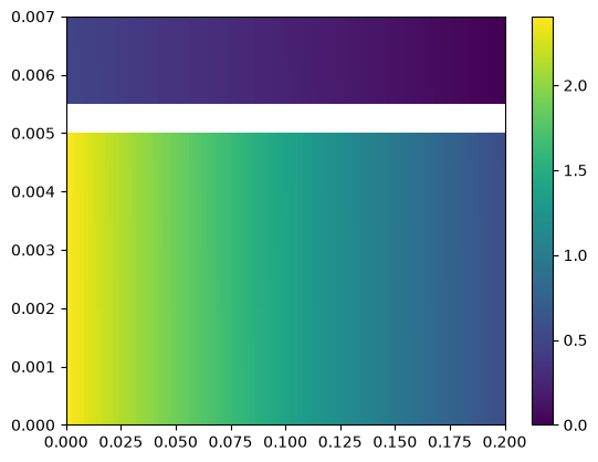

retentate side: inlet molar flow = 1.88934e-06, membrane molar flow out = 1.44650e-06, outlet molar flow = 4.42837e-07
retentate balance: -4.02605e-19
permeate side:  inlet molar flow = 0.00000e+00, membrane molar flow in  = 1.44650e-06, outlet molar flow = 1.44650e-06
permeate balance: 5.32784e-19
overall balance: -6.01182e-19

Checking the result¶

describe_bc prints a boundary-condition dictionary as the equation it actually imposes. ic_1_neumann and ic_2_neumann couple both fields, so a lists the retentate and permeate coefficients in order. As in the plain membrane model, the two conditions look alike, but because pymrm boundary conditions always use the outward normal (pitfall P1), the sign of the flux term flips between the retentate (inner, upper $r$ boundary) and permeate (outer, lower $r$ boundary) sides.

from pymrm import describe_bc

print("Retentate side interface condition (ic_1_neumann):")
print(describe_bc((bc_neumann, ic_1_neumann), r_f_ret, axis_name="r", var="c"))
print()
print("Permeate side interface condition (ic_2_neumann):")
print(describe_bc((ic_2_neumann, bc_neumann), r_f_perm, axis_name="r", var="c"))

Retentate side interface condition (ic_1_neumann):
lower (r=0, outward normal -r): -1*dc/dr + 0*c = 0  [Neumann]
upper (r=0.005, outward normal +r): [0.0001, 0]*dc/dr + 0*c = 5e-06  [mixed or degenerate]

Permeate side interface condition (ic_2_neumann):
lower (r=0.0055, outward normal -r): [0, -0.00011]*dc/dr + 0*c = -5e-06  [mixed or degenerate]
upper (r=0.007, outward normal +r): 1*dc/dr + 0*c = 0  [Neumann]