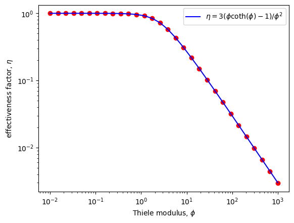
Particle model: diffusion + first order reaction - Multiphase Reactor Modeling using PyMRM

This notebook demonstrates how to compute the effectiveness factor of a particle model with diffusion and a first-order reaction.

A non-uniform grid is used, refined near the particle surface, to ensure accurate computation for larger Thiele moduli.

The governing equation for the dimensionless concentration $c$ in a spherical particle of radius $R$ , with diffusion coefficient $D$ and a first-order reaction with rate constant $k$ , is

D \frac{1}{r^2}\frac{d}{dr}\left(r^2 \frac{dc}{dr}\right) = k c.

(1)

The boundary conditions are symmetry (no flux) at the particle centre, $dc/dr = 0$ at $r=0$ , and a fixed surface concentration, $c=1$ at $r=R$ . In pymrm’s a*dc/dn + b*c = d convention, with $n$ the outward normal, the outward normal at the lower end ( $r=0$ ) points in the $-r$ direction, so {'a':1, 'b':0, 'd':0} there imposes $-dc/dr=0$ , i.e. the intended symmetry condition; at the upper end ( $r=R$ ) the outward normal is $+r$ , so {'a':0, 'b':1, 'd':1} imposes $c=1$ .

# Import required libraries
import matplotlib.pyplot as plt
from pymrm import non_uniform_grid

# Define grid parameters
shape_c = (30,)  # Number of cells in the grid
R = 1  # Radius of the particle
dr_large = 0.1*R  # Initial large spacing for the grid

# Generate a non-uniform grid refined near the particle surface
r_f = non_uniform_grid(0, R, shape_c[0]+1, dr_large, 0.75)

# Plot the non-uniform grid positions
plt.plot(r_f, marker = 'o', linestyle = '')
plt.title("non-uniform grid positions")
plt.xlabel("number")
plt.ylabel("position of cell faces")
plt.show()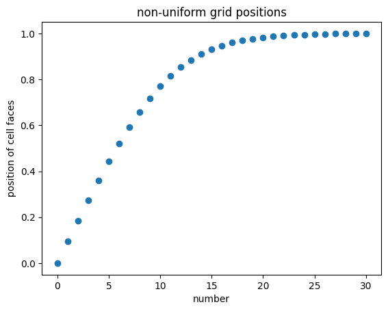

Parameters and operators¶

Define the diffusion coefficient, the sweep of Thiele moduli, and the boundary conditions, then build the gradient, divergence, and Laplacian operators on the non-uniform grid.

# Import required libraries
import math
import numpy as np
from scipy.sparse import eye_array
from scipy.sparse import linalg as sla
import matplotlib.pyplot as plt
from pymrm import construct_grad, construct_div

# Define constants and parameters
D = 1  # Diffusion coefficient
phis = np.logspace(-2,3,30)  # Range of Thiele moduli
bc = ({'a':1 , 'b':0, 'd':0},{'a':0, 'b':1, 'd':1})  # Boundary conditions

# Construct gradient and divergence matrices
grad_mat, grad_bc = construct_grad(shape_c, r_f, bc=bc)
div_mat = construct_div(shape_c, r_f, nu=2, axis=0)

# Compute Laplacian matrix and boundary conditions
lapl_mat = div_mat @ grad_mat
lapl_bc = div_mat @ grad_bc

Effectiveness factor sweep¶

For each Thiele modulus, build and factorize the Jacobian, solve for the concentration profile, and compute the apparent reaction rate from the surface gradient to obtain the effectiveness factor. The analytical closed form for a sphere is plotted for comparison.

# Loop over Thiele moduli to compute effectiveness factor
for phi in phis:
    k = phi**2*D/R  # Reaction rate constant
    jac = k*eye_array(math.prod(shape_c), format='csc') - lapl_mat  # Jacobian matrix
    jac_lu = sla.splu(jac)  # LU decomposition of the Jacobian

    # Solve for concentration profile
    c = jac_lu.solve(lapl_bc.toarray())
    k_app = (grad_mat[[-1],:] @ c + grad_bc[[-1]].toarray())[[0]]*(3*D/R)  # Apparent reaction rate
    eta = k_app/k  # Effectiveness factor
    c = c.reshape(shape_c)  # Reshape concentration profile

    # Plot effectiveness factor for the current Thiele modulus
    plt.loglog(phi, eta, marker = 'o', linestyle = '', color = 'red')

# Plot analytical solution for comparison
plt.loglog(phis, 3*(phis/np.tanh(phis)-1)/(phis*phis), color = 'blue', label = r'$\eta = 3(\phi \coth(\phi)-1)/\phi^2$')
plt.xlabel(r'Thiele modulus, $\phi$')
plt.ylabel(r'effectiveness factor, $\eta$')
plt.legend()
plt.show()

Checking the result¶

The plot above already compares the numerical effectiveness factor against the sphere’s analytical closed form $\eta = 3(\phi \coth(\phi)-1)/\phi^2$ . Here the comparison is quantified: the numerical values should match the analytical ones to within the discretization error. A large mismatch here would catch a wrong divergence operator (nu), a wrong sign in the boundary conditions, or a wrong apparent-rate formula.

# Recompute eta for each phi, reusing the operators built above, and compare against the analytical formula
from pymrm import describe_bc

eta_num = np.zeros_like(phis)
for i, phi in enumerate(phis):
    k = phi**2*D/R
    jac = k*eye_array(math.prod(shape_c), format='csc') - lapl_mat
    jac_lu = sla.splu(jac)
    c_i = jac_lu.solve(lapl_bc.toarray())
    k_app = (grad_mat[[-1],:] @ c_i + grad_bc[[-1]].toarray())[[0]]*(3*D/R)
    eta_num[i] = np.asarray(k_app/k).reshape(-1)[0]

eta_analytical = 3*(phis/np.tanh(phis)-1)/(phis*phis)

# Away from phi -> 0 (where eta -> 1 and relative error becomes noisy), compare on the rest of the sweep
mask = phis > 0.1
rel_err = np.abs(eta_num[mask] - eta_analytical[mask])/eta_analytical[mask]
print(f"max relative error (phi > 0.1): {rel_err.max():.3e}")

abs_err_small = np.abs(eta_num[~mask] - eta_analytical[~mask])
print(f"max absolute error (phi <= 0.1): {abs_err_small.max():.3e}")

for line in describe_bc(bc, r_f).splitlines():
    print(line)

max relative error (phi > 0.1): 1.522e-02
max absolute error (phi <= 0.1): 1.537e-06
lower (x=0, outward normal -x): -1*dc/dx + 0*c = 0  [Neumann]
upper (x=1, outward normal +x): 0*dc/dx + 1*c = 1  [Dirichlet]