Counter-current convection and reaction - Multiphase Reactor Modeling using PyMRM

Reaction: $A+B\rightarrow *$

$\frac{\partial c_A}{\partial t} + \mathrm{div}(v_A \, c_A) = -k \, c_A c_B$

$\frac{\partial c_B}{\partial t} + \mathrm{div}(v_B \, c_B) = -k \, c_A c_B$

with boundary conditions: $c_A(0)=1$ , $\frac{\partial c_A(L)}{\partial n} = 0$ , $\frac{\partial c_B(0)}{\partial n} = 0$ , $c_B(L)=1$

Notes:

Counter-current flow is implemented by taking $v_B$ negative and setting the proper boundary conditions.
With $|v_A| > |v_B|$ and same inlet concentrations not all $A$ will react away.
For high reaction rate coefficient $k$ , there is only a thin boundary layer where $B$ is present. If this boundary layer is not resolved the result is incorrect. Uncomment the non-uniform mesh for high $k$ .
This is a numerically tough problem for high reaction rates. Note that TVD deferred correction is currently off, i.e. the upwind scheme is used. TVD seems to decrease robustness.

Imports¶

import numpy as np
from scipy.sparse import eye_array, linalg as sla
import matplotlib.pyplot as plt
from IPython.display import clear_output, display
from pymrm import (
    non_uniform_grid,
    construct_convflux_upwind,
    construct_div,
    NumJac,
    interp_cntr_to_stagg_tvd,
    upwind,
    minmod,
)

Parameters and boundary conditions¶

Physical and numerical parameters, and the boundary dictionaries in the a*dc/dn + b*c = d convention (outward normal): a Danckwerts-style inlet for $A$ at $x=0$ with a zero-gradient outlet at $x=L$ , and the mirror image for $B$ .

# Physical parameters and boundary conditions
num_c = 2
L = 1.0
k = 100
v = [[1, -0.5]]
bc_L = {'a': [[0, 1]], 'b': [[1, 0]], 'd': [[1, 0]]}
bc_R = {'a': [[1, 0]], 'b': [[0, 1]], 'd': [[0, 1]]}
bc = (bc_L, bc_R)

# Numerical parameters
dt = 1
num_time_steps = 100
num_inner_iter = 2
num_x = 100
shape = (num_x, num_c)

Reaction term¶

$A + B \rightarrow *$ with rate $k \, c_A c_B$ , consuming $A$ and $B$ in equal amounts.

def reaction(c, k):
    f = np.empty_like(c)
    r = k * c[:, 0] * c[:, 1]
    f[:, 0] = -r
    f[:, 1] = -r
    return f

Grid and operators¶

A grid refined near both ends (needed to resolve the thin reaction layer at high $k$ ) and the constant convection and divergence operators. The first-order upwind part of the convection is kept in the constant Jacobian; a TVD deferred correction is added explicitly in the solve loop.

#x_f = np.linspace(0, L, num_x + 1)
x_f = non_uniform_grid(0, L, shape[0] + 1, 0.05 * L, 0.75)
x_c = 0.5 * (x_f[:-1] + x_f[1:])

conv_mat, conv_bc = construct_convflux_upwind(shape, x_f, x_c, bc, v, axis=0)
div_mat = construct_div(shape, x_f, nu=0, axis=0)
g_const = div_mat @ conv_bc
jac_const = eye_array(np.prod(shape), format='csc') / dt + div_mat @ conv_mat
numjac_react = NumJac(shape, axes_blocks=[-1])

Solve (pseudo-transient Newton)¶

Implicit Euler time stepping toward steady state; each step takes num_inner_iter Newton iterations with the reaction Jacobian rebuilt from NumJac and the TVD deferred correction added to the residual. TVD is currently off (plain upwind is used); switch interp_cntr_to_stagg_tvd’s limiter argument to minmod to turn it back on, at the cost of robustness for this stiff reaction.

c = np.zeros(shape)
for i in range(num_time_steps):
    c_old = c.copy()
    for j in range(num_inner_iter):
        f_react, jac_react = numjac_react(lambda c: reaction(c, k), c)
        jac = jac_const - jac_react
        jac_lu = sla.splu(jac)
        c_f, dc_f = interp_cntr_to_stagg_tvd(c, x_f, x_c, bc, v, upwind, axis=0)
#        c_f, dc_f = interp_cntr_to_stagg_tvd(c, x_f, x_c, bc, v, minmod, axis=0)
        g_conv_deferred = div_mat @ (v * dc_f).reshape((-1, 1))
        g = (
            -c_old.reshape(-1, 1) / dt
            + jac_const @ c.reshape(-1, 1)
            + g_conv_deferred
            + g_const
            - f_react.reshape(-1, 1)
        )
        c -= jac_lu.solve(g).reshape(c.shape)
    clear_output(wait=True)
    display(f'progress: {i + 1} out of {num_time_steps}')

'progress: 100 out of 100'

Plot the concentration profiles¶

fig, ax = plt.subplots()
line0, = ax.plot(x_c, c[:, 0])
line1, = ax.plot(x_c, c[:, 1])
ax.set_xlabel('Position')
ax.set_ylabel('Concentration')
fig.canvas.draw()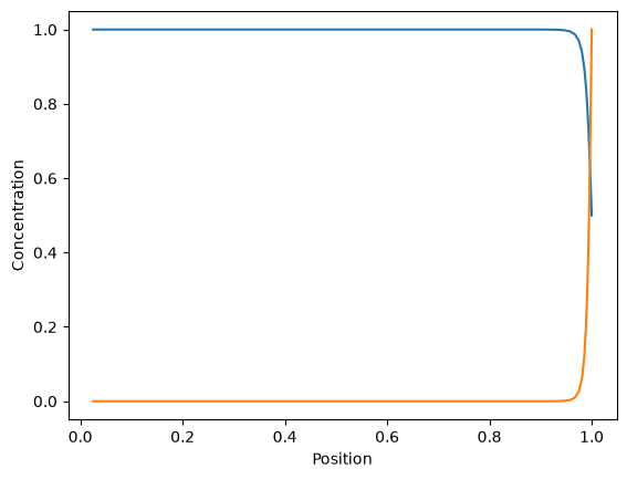

Checking the result¶

$A$ enters at $x=0$ with velocity $v_A=1$ and $B$ enters at $x=L$ with velocity $|v_B|=0.5$ (counter-current); at steady state the net convective inflow of $A$ must equal the amount consumed by the reaction, $v_A\,[c_A(0)-c_A(L)] = \int_0^L k\,c_Ac_B\,dx$ , read from the FACE values with compute_boundary_values (not the last cell centre). This catches a wrong boundary-condition sign, a reaction term left out of the residual, or a run that has not actually reached steady state.

from pymrm import compute_boundary_values

c_lo, _, c_hi, _ = compute_boundary_values(c, x_f, x_c, bc, axis=0)
v_arr = np.asarray(v).reshape(1, -1)
dz = np.diff(x_f)
consumed = np.sum(k * c[:, 0] * c[:, 1] * dz)

flux_in_a = v_arr[0, 0] * c_lo[0, 0]
flux_out_a = v_arr[0, 0] * c_hi[0, 0]
balance_a = flux_in_a - flux_out_a - consumed
print(f"A: inflow {flux_in_a:.6f}, outflow {flux_out_a:.6f}, consumed {consumed:.6f}, "
      f"balance residual {balance_a:.3e}")
print("A closed balance to machine precision confirms the steady state and the reaction term are consistent." if abs(balance_a) < 1e-8 * consumed else "Balance does not close: check convergence or the reaction/BC assembly.")

A: inflow 1.000000, outflow 0.500000, consumed 0.500000, balance residual 0.000e+00
A closed balance to machine precision confirms the steady state and the reaction term are consistent.