Heat conduction around solid particles: grid convergence of the immersed boundary method

A fluid of thermal conductivity $k$ occupies a square domain containing solid particles (disks). At every particle surface a Robin (contact-conductance) condition couples the outward heat flux to the surface temperature,

k\,\frac{\partial T}{\partial n_\text{out}} + h\,T_\Gamma \;=\; d ,

(1)

with $h$ a surface heat-transfer coefficient and $n_\text{out}$ the outward (fluid-side) direction. We solve the steady conduction equation $-\nabla\!\cdot\!(k\nabla T) = q$ and study the grid convergence of the immersed-boundary discretisation — in particular what happens when two particles touch.

The same physical problem is discretised in two ways:

Full SDF description — the classical route: one global signed-distance field sdf = min_i(dist_i) sampled at the cell centres; construct_ibm(sdf, ...) locates the walls by linear interpolation of the SDF and construct_ibm_normal_derivative takes the surface normals from the SDF gradient.
Particle description — the circles are described analytically by pymrm.Circle objects; construct_ibm_particles computes exact wall positions (quadratic solve per cut face) and exact outward normals.

A manufactured temperature field $T^{\ast}$ defines the source $q$ , the domain wall temperatures, and the Robin data $d$ , so the exact solution is known on every grid for any particle arrangement — including exact contact, where no analytic solution exists.

1. Manufactured solution and helpers¶

T^{\ast}(x,y) = 300 + 20\cos(1.3\pi x)\cos(0.8\pi y) + 8x + 5y \quad [\mathrm{K}]

(2)

with $k = 2.5\ \mathrm{W\,m^{-1}K^{-1}}$ and $h = 8\ \mathrm{W\,m^{-2}K^{-1}}$ . The volumetric source is $q = -k\nabla^2 T^{\ast}$ ; the domain walls are held at $T^{\ast}$ ; the Robin data is $d = k\,\partial T^{\ast}/\partial n_\text{out} + h\,T^{\ast}$ evaluated at the wall crossings with the exact geometric normal — the problem data is identical for both discretisations, only the geometric information inside the method differs.

import warnings
warnings.filterwarnings("ignore")
import numpy as np
import matplotlib.pyplot as plt
from scipy.sparse import csc_array
from scipy.sparse.linalg import spsolve

from pymrm import (construct_grad, construct_div, construct_ibm, apply_ibm,
                   apply_ibm_vector, construct_ibm_normal_derivative,
                   construct_ibm_boundary_values, Circle,
                   construct_ibm_particles)
from pymrm.ibm_recon import interface_normals

K_COND = 2.5      # fluid thermal conductivity  [W/m/K]
H_SURF = 8.0      # surface heat-transfer coefficient  [W/m^2/K]
KX, KY = 1.3 * np.pi, 0.8 * np.pi
Ns = [40, 80, 160, 320]          # grid sequence (reduce for a faster run)

def T_star(x, y):
    return 300.0 + 20.0 * np.cos(KX * x) * np.cos(KY * y) + 8.0 * x + 5.0 * y

def grad_T_star(x, y):
    return (-20.0 * KX * np.sin(KX * x) * np.cos(KY * y) + 8.0,
            -20.0 * KY * np.cos(KX * x) * np.sin(KY * y) + 5.0)

def source(x, y):                        # q = -k lap T*
    return 20.0 * K_COND * (KX**2 + KY**2) * np.cos(KX * x) * np.cos(KY * y)

def make_grid(N):
    x_f = [np.linspace(0.0, 1.0, N + 1), np.linspace(0.0, 1.0, N + 1)]
    x_c = [0.5 * (xf[:-1] + xf[1:]) for xf in x_f]
    X, Y = np.meshgrid(x_c[0], x_c[1], indexing="ij")
    return x_f, x_c, X, Y

def err_norms(T, T_ex, fluid, h):
    e = (T - T_ex)[fluid]
    return (np.sum(np.abs(e)) * h * h,
            np.sqrt(np.sum(e**2) * h * h),
            np.abs(e).max())

def order(errs):
    return [float("nan")] + [np.log(errs[k-1] / errs[k]) / np.log(2)
                             for k in range(1, len(errs))]

def report(label, results):
    print(f"\n=== {label} ===")
    print(f"{'N':>5} {'L1':>11} {'ord':>5} {'L2':>11} {'ord':>5} "
          f"{'Linf':>11} {'ord':>5}")
    o1, o2, oi = (order([r[j] for r in results]) for j in range(3))
    for k, N in enumerate(Ns):
        print(f"{N:>5} {results[k][0]:>11.3e} {o1[k]:>5.2f} "
              f"{results[k][1]:>11.3e} {o2[k]:>5.2f} "
              f"{results[k][2]:>11.3e} {oi[k]:>5.2f}")
    return [r[1] for r in results]        # L2 errors for the figure

2. Geometries¶

A single disk, and two disks in exact contact. Both are defined once as (centre, radius) pairs; the SDF route derives the union field from them, the particle route wraps them in analytic Circle objects. The exact outward normal of the owning disk provides the Robin problem data in both cases.

DISKS_SINGLE = [((0.503, 0.497), 0.28)]
R_T = 0.22
DISKS_TOUCH = [((0.5 - R_T, 0.5015), R_T), ((0.5 + R_T, 0.5015), R_T)]

def union_sdf(disks, X, Y):
    return np.minimum.reduce(
        [np.hypot(X - cx, Y - cy) - r for (cx, cy), r in disks])

def exact_normals(coords, disks):
    '''Outward unit normal of the disk whose surface is nearest.'''
    n = np.zeros_like(coords)
    best = np.full(len(coords), np.inf)
    for (cx, cy), r in disks:
        dist = np.abs(np.hypot(coords[:, 0] - cx, coords[:, 1] - cy) - r)
        take = dist < best
        best[take] = dist[take]
        v = coords[take] - np.array([cx, cy])
        n[take] = v / np.linalg.norm(v, axis=1, keepdims=True)
    return n

3. Shared discretisation¶

One solver serves both geometry descriptions. It receives the immersed boundary data (ibm), a field for fluid/solid classification in the reconstruction, and optionally overriding normals; everything else — the conduction operator $-\nabla\cdot(k\nabla T)$ with Dirichlet $T^{\ast}$ domain walls, identity rows in the (unmodelled) solid, the GFD flux reconstruction, and the Robin elimination — is identical:

A\,T = b, \qquad A = A_\text{ibm} + G_\text{out} H,

(3)

with $H$ from construct_ibm_boundary_values expressing the surface temperature $T_\Gamma$ in terms of the fluid field.

def solve_heat(N, disks, geometry):
    '''geometry(N, disks) -> (ibm, sdf_for_recon, normals_or_None, solid_mask)'''
    x_f, x_c, X, Y = make_grid(N)
    ibm, sdf_recon, normals, solid = geometry(N, disks)

    # conduction operator with Dirichlet T* domain walls
    shape = (N, N)
    diff = csc_array((N * N, N * N)); g_bc = np.zeros((N * N, 1))
    for i in range(2):
        if i == 0:
            bc = ({'a': 0, 'b': 1, 'd': T_star(0.0, x_c[1])[None, :]},
                  {'a': 0, 'b': 1, 'd': T_star(1.0, x_c[1])[None, :]})
        else:
            bc = ({'a': 0, 'b': 1, 'd': T_star(x_c[0], 0.0)[:, None]},
                  {'a': 0, 'b': 1, 'd': T_star(x_c[0], 1.0)[:, None]})
        gm, gb = construct_grad(shape, x_f[i], x_c[i], bc=bc, axis=i, format='csc')
        dv = construct_div(shape, x_f[i], axis=i, format='csc')
        diff = diff + dv @ (-K_COND * gm)
        g_bc = g_bc + dv @ (-K_COND * gb)
    g_bc = np.asarray(g_bc).reshape(-1)
    q = source(X, Y).reshape(-1)

    fluid = ~solid.reshape(-1)
    diff = diff.tolil()                       # unmodelled solid -> identity rows
    for r in np.flatnonzero(~fluid):
        diff.rows[r] = [r]; diff.data[r] = [1.0]
    diff = diff.tocsc()
    rhs0 = np.where(fluid, q - g_bc, 0.0)

    # flux reconstruction + Robin elimination at the particle surfaces
    recon = construct_ibm_normal_derivative(ibm, sdf_recon, x_c, normals=normals)
    ne = exact_normals(ibm.coords, disks)     # problem data: exact geometry
    gx, gy = grad_T_star(ibm.coords[:, 0], ibm.coords[:, 1])
    q_out_star = -(gx * ne[:, 0] + gy * ne[:, 1])
    d_rob = K_COND * q_out_star + H_SURF * T_star(ibm.coords[:, 0],
                                                  ibm.coords[:, 1])

    A_ibm, G_out, G_in = apply_ibm(diff, ibm, return_bc="matrix")
    H, h_vec = construct_ibm_boundary_values(
        ibm, recon, {'a': K_COND, 'b': H_SURF, 'd': d_rob}, side='out')
    A = (A_ibm + G_out @ H).tocsr()
    b = apply_ibm_vector(rhs0, ibm) - np.asarray(G_out @ h_vec).ravel()
    T = spsolve(A.tocsc(), b)
    return err_norms(T, T_star(X, Y).reshape(-1), fluid, 1.0 / N)

4. Method 1 — full SDF description¶

The union SDF is sampled at the cell centres; wall positions come from linear interpolation of the SDF along each cut face, and the surface normals from the interpolated SDF gradient (interface_normals, the library default).

def geometry_sdf(N, disks):
    x_f, x_c, X, Y = make_grid(N)
    sdf = union_sdf(disks, X, Y)
    ibm = construct_ibm(sdf, x_c)
    return ibm, sdf, None, (sdf < 0)

res_sdf_single = [solve_heat(N, DISKS_SINGLE, geometry_sdf) for N in Ns]
res_sdf_touch = [solve_heat(N, DISKS_TOUCH, geometry_sdf) for N in Ns]
L2_sdf_single = report("SDF  |  single disk", res_sdf_single)
L2_sdf_touch = report("SDF  |  two touching disks", res_sdf_touch)


=== SDF  |  single disk ===
    N          L1   ord          L2   ord        Linf   ord
   40   3.679e-03   nan   5.887e-03   nan   2.824e-02   nan
   80   8.819e-04  2.06   1.391e-03  2.08   5.806e-03  2.28
  160   2.165e-04  2.03   3.443e-04  2.01   1.364e-03  2.09
  320   5.568e-05  1.96   8.835e-05  1.96   3.582e-04  1.93

=== SDF  |  two touching disks ===
    N          L1   ord          L2   ord        Linf   ord
   40   1.480e-02   nan   4.018e-02   nan   5.509e-01   nan
   80   7.756e-03  0.93   2.406e-02  0.74   5.087e-01  0.11
  160   3.286e-03  1.24   1.116e-02  1.11   3.695e-01  0.46
  320   1.339e-03  1.29   5.073e-03  1.14   2.585e-01  0.52

The single disk converges at the expected 2nd order. For the touching disks the order collapses to ~1 in L2 (and ~0.5 in the maximum norm): the union SDF is not differentiable on the contact medial axis, so the SDF-gradient normals carry an O(1) error in a fixed cluster of crossings at the contact, and the interpolated wall positions there are polluted by the other disk’s distance field.

5. Method 2 — analytic particle description¶

The same disks as Circle particles: construct_ibm_particles classifies the cells per particle (bounding-box windows), computes each cut-face wall position exactly (quadratic solve on the owning circle) and returns the exact outward normals in info.normals. The info.pseudo_sdf field (sign-correct union) serves the fluid/solid classification of the reconstruction; sub-cell gaps at the contact are walled off by the default contact="no_flux" policy (inert here, since the solid is not modelled).

def geometry_particles(N, disks):
    x_f, x_c, X, Y = make_grid(N)
    parts = [Circle(c, r) for c, r in disks]
    ibm, info = construct_ibm_particles(parts, x_c)
    return ibm, info.pseudo_sdf, info.normals, (info.owner >= 0)

res_p_single = [solve_heat(N, DISKS_SINGLE, geometry_particles) for N in Ns]
res_p_touch = [solve_heat(N, DISKS_TOUCH, geometry_particles) for N in Ns]
L2_p_single = report("Particles  |  single disk", res_p_single)
L2_p_touch = report("Particles  |  two touching disks", res_p_touch)


=== Particles  |  single disk ===
    N          L1   ord          L2   ord        Linf   ord
   40   3.839e-03   nan   6.122e-03   nan   2.903e-02   nan
   80   9.214e-04  2.06   1.451e-03  2.08   5.993e-03  2.28
  160   2.258e-04  2.03   3.580e-04  2.02   1.400e-03  2.10
  320   5.791e-05  1.96   9.170e-05  1.96   3.677e-04  1.93

=== Particles  |  two touching disks ===
    N          L1   ord          L2   ord        Linf   ord
   40   3.542e-03   nan   7.599e-03   nan   1.408e-01   nan
   80   8.649e-04  2.03   1.907e-03  1.99   5.151e-02  1.45
  160   2.474e-04  1.81   5.998e-04  1.67   2.410e-02  1.10
  320   6.433e-05  1.94   1.639e-04  1.87   1.001e-02  1.27

The particle description leaves the single disk unchanged (~2nd order, marginally smaller constants from the exact walls) and restores the touching case to ~1.8 in L2, reducing the error by more than an order of magnitude on the finer grids.

6. Convergence comparison¶

h = np.array([1.0 / N for N in Ns])
fig, ax = plt.subplots(1, 2, figsize=(11, 4.6), sharey=True)

for a, (l_sdf, l_p, title) in zip(
        ax, [(L2_sdf_single, L2_p_single, "single disk"),
             (L2_sdf_touch, L2_p_touch, "two touching disks")]):
    a.loglog(h, l_sdf, 's-', color='tab:red', label='full SDF')
    a.loglog(h, l_p, '^-', color='tab:green', label='analytic particles')
    a.loglog(h, l_p[0] * (h / h[0])**2, 'k--', lw=1, label='slope 2')
    a.loglog(h, l_sdf[0] * (h / h[0])**1, 'k:', lw=1, label='slope 1')
    a.set(xlabel='h', title=title)
    a.grid(True, which='both', alpha=0.3)
ax[0].set_ylabel(r'L2 temperature error  [K$\cdot$m]')
ax[0].legend(fontsize=8)
fig.suptitle('Immersed-boundary heat conduction: SDF vs particle description')
fig.tight_layout(); plt.show()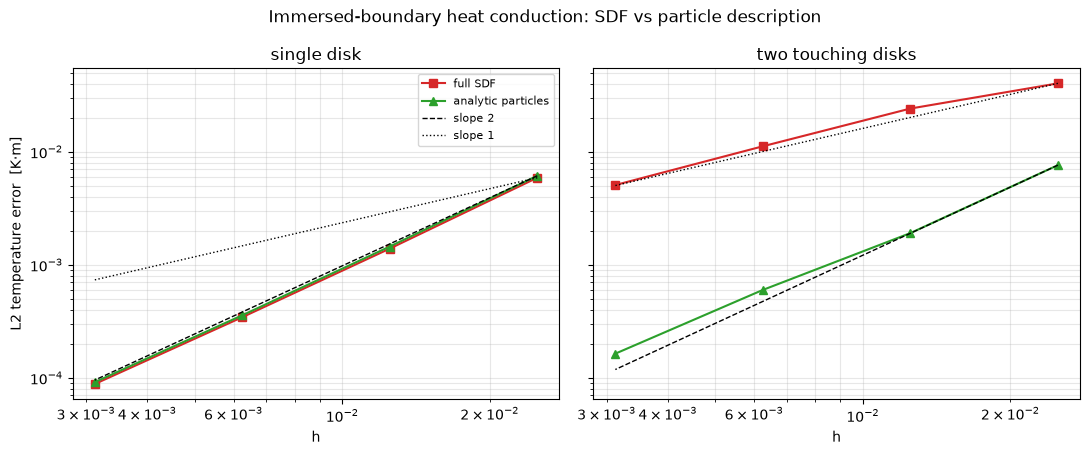

7. Where the difference comes from¶

Two localized geometry errors of the SDF route at the contact, neither of which is a stencil problem:

Normals — the union SDF has a gradient kink on the contact medial axis; differencing across it tilts the normals by an O(1) angle in a fixed cluster of crossings (only shrinking as O(h) with resolution). The analytic particle normals are exact.
Wall positions — the interpolated theta uses the union value at the ghost cell, which near the contact belongs to the other disk. The particle route intersects each face with the owning circle exactly.

The GFD flux stencils themselves stay healthy (hardly any degree demotion, no unresolved crossings):

for N in Ns:
    x_f, x_c, X, Y = make_grid(N)
    sdf = union_sdf(DISKS_TOUCH, X, Y)
    ibm = construct_ibm(sdf, x_c)
    parts = [Circle(c, r) for c, r in DISKS_TOUCH]
    ibm_p, info = construct_ibm_particles(parts, x_c)
    reg = ~info.contact          # regular crossings: on a particle surface
    # (contact crossings sit at the mid-gap point by construction and their
    #  normal points towards the partner particle - excluded here)

    ne = exact_normals(ibm.coords, DISKS_TOUCH)
    ang = lambda a, b: np.degrees(np.arccos(np.clip(np.sum(a * b, 1), -1, 1)))
    a_sdf = ang(interface_normals(ibm, sdf, x_c), ne)
    a_p = ang(info.normals[reg],
              exact_normals(ibm_p.coords[reg], DISKS_TOUCH))
    on_circle = np.minimum.reduce(
        [np.abs(np.hypot(ibm_p.coords[reg, 0] - cx,
                         ibm_p.coords[reg, 1] - cy) - r)
         for (cx, cy), r in DISKS_TOUCH])
    recon = construct_ibm_normal_derivative(ibm, sdf, x_c)
    print(f"N={N:4d}  normal err (deg): sdf max {a_sdf.max():6.2f}"
          f"  particles max {a_p.max():.1e}   "
          f"particle wall off-surface: {on_circle.max():.1e}   "
          f"degree<2: {int((recon.degree_out < 2).sum())}, "
          f"unresolved: {int(recon.unresolved_out.sum())}")

N=  40  normal err (deg): sdf max  15.62  particles max 1.2e-06   particle wall off-surface: 8.3e-17   degree<2: 6, unresolved: 0
N=  80  normal err (deg): sdf max  12.23  particles max 1.5e-06   particle wall off-surface: 8.3e-17   degree<2: 8, unresolved: 0

N= 160  normal err (deg): sdf max   9.13  particles max 1.2e-06   particle wall off-surface: 8.3e-17   degree<2: 8, unresolved: 0

N= 320  normal err (deg): sdf max   6.63  particles max 1.5e-06   particle wall off-surface: 8.3e-17   degree<2: 8, unresolved: 0

8. What the particle description provides beyond accuracy¶

At exact contact the two disks share solid cells, so a segmentation of the union SDF sees one body. The particle assembly keeps per-particle ownership: info.segmentation labels the disks separately (enabling per-particle surface conditions), and the sub-cell gap faces detected at the contact are walled off by the default no_flux policy — if the solid interiors were modelled (conjugate heat transfer), no matrix entry would couple the two particles directly:

x_f, x_c, X, Y = make_grid(64)
parts = [Circle(c, r) for c, r in DISKS_TOUCH]
ibm_c, info_c = construct_ibm_particles(parts, x_c)
print('contact crossings walled off :', int(info_c.contact.sum()))
print('per-particle segment sizes   :', info_c.segmentation.sizes)

L = csc_array((64 * 64, 64 * 64))
for a in range(2):
    gm, _ = construct_grad((64, 64), x_f[a], x_c[a], axis=a, format='csc')
    dv = construct_div((64, 64), x_f[a], axis=a, format='csc')
    L = L + dv @ gm
A, _ = apply_ibm(L.tocsr(), ibm_c, values_outside=0.0, values_inside=0.0)
own = info_c.owner.ravel()
block = A[np.ix_(np.flatnonzero(own == 0), np.flatnonzero(own == 1))]
print('max |coupling| disk-1 rows x disk-2 cols:', np.abs(block).max())

contact crossings walled off : 8
per-particle segment sizes   : [622 622]
max |coupling| disk-1 rows x disk-2 cols: 0.0

9. Summary¶

case	full SDF	analytic particles
single disk	~2.0	~2.0
two touching disks (L2)	~1.0	~1.8

The immersed Robin/flux discretisation is 2nd order for isolated particles under either description.
At particle contact the full-SDF route degrades to ~1st order through purely geometric errors (kinked-gradient normals, polluted wall positions), not stencil failure.
The analytic particle description removes both error sources and restores ~1.8 (L2) / ~1.25 (L∞); the residual gap to 2 is a genuine PDE singularity of the re-entrant contact corner, beyond any fixed-stencil scheme.
The particle route additionally provides per-particle segmentation at contact and the no_flux contact policy for conjugate problems.
(The Dirichlet ghost-cell method apply_ibm is insensitive to all of this — it is 2nd order even for touching particles, as it uses no normals.)