# Bootstrap: the pymrm this page was checked with, and the gallery files it was
# published with. Works in a checkout, in CI and on a fresh Colab VM.
GALLERY_REF = "gallery-2026.11.10.3"  # replaced by the release tag at publication
PYMRM = ">=3.4.0,<4"  # equals meta.yaml pymrm_min_version, up to the next major
PAGE = "A2.6-gunn-dispersion-correlations"  # equals the page directory

import os, sys, urllib.request
from pathlib import Path
_shared = next((p / "shared" for p in (Path.cwd(), *Path.cwd().parents)
                if (p / "shared" / "gallery_bootstrap.py").is_file()), None)
if _shared is None:
    _shared = (Path(os.environ.get("XDG_CACHE_HOME") or Path.home() / ".cache")
               / "pymrm-gallery" / GALLERY_REF)
    _shared.mkdir(parents=True, exist_ok=True)
    urllib.request.urlretrieve(
        "https://raw.githubusercontent.com/computational-chemical-engineering/"
        f"pymrm-gallery/{GALLERY_REF}/shared/gallery_bootstrap.py",
        _shared / "gallery_bootstrap.py")
sys.path.insert(0, str(_shared))
sys.modules.pop("gallery_bootstrap", None)
from gallery_bootstrap import setup
setup(PAGE, PYMRM, GALLERY_REF); # the semicolon stops the cell echoing the pathGunn’s dispersion correlations, and what the number 2 depends on
sec:A
struct:S6
tier:T1
data:tier2
phase:gas
The stochastic fast/slow-stream model for axial and radial dispersion in fixed beds, its one empirical function p(Re), and a 2-D pymrm bed that uses both coefficients at once.
Gunn’s dispersion correlations, and what the number 2 depends on
Catalog ID: A2.6 · Structures: S6 (2-D axisymmetric dispersion–reaction) · Tier: T1
Three gallery pages already touch the axial-dispersion coefficient. A2.1 takes it as given and asks what its boundary conditions mean; A2.3 derives one for an empty tube; A2.5 measures one in a packed bed and fits a two-constant correlation to the measurement.
This page is the fourth question. Gunn’s model is not a curve fit: it is a stochastic argument about a molecule moving between a fast and a slow stream, with one empirical function in it, and it covers axial and radial dispersion, spheres and cylinders, gases and liquids, over a 2000-fold range of Schmidt group. That breadth is what makes it testable, and it is what lets the page ask a question A2.5 cannot: where does the “widely quoted value of 2” come from, and is it a law or a coincidence?
import re
from functools import lru_cache

import numpy as np
import pandas as pd
import matplotlib.pyplot as plt
import mpmath as mp
from IPython.display import Markdown, display
from scipy.integrate import solve_bvp
from scipy.optimize import minimize_scalar
from pymrm import describe_bc
from pymrm.checks import find_roots, observed_orders
from gallery_utils import load_data, load_meta, cite_data, load_claims, Claims
from model import (ALPHA1, BETA1, SHAPES, Bed, D_over_Ud, D_over_Ud_1993,  # this page's model.py
                   Pe_axial, Pe_f, Pe_radial, dD_over_Ud_dRe, p_of_Re)

plt.rcParams.update({"figure.dpi": 110, "axes.grid": True, "grid.alpha": 0.3})
claims = Claims(PAGE.split("-")[0])
A25 = "A2.5-edwards-richardson-dispersion"


# Deviations are reported ONE way everywhere on this page:
#     dev = (model - reference) / reference
def dev(model, reference):
    return np.asarray(model, float) / np.asarray(reference, float) - 1.0
Background
A tracer molecule in a packed bed is doing two things at once. It is carried downstream by the fluid, at a speed that depends on which part of the pore space it happens to be in; and it diffuses between those parts. Gunn’s model, developed in his 1969 Trans. IChemE paper and summarised in the 1987 one this page is built from, makes that literal. In a characteristic time \(d/U\) a molecule either moves one particle diameter downstream, with probability \(p\), or it does not. Molecular diffusion moves it between the fast and the slow region. \(p\) is identified with “the relative proportions of the moving region of fluid in a cell of particles to the slow moving or static regions of fluid”.
Everything else in the resulting expression is geometry or molecular physics. There is exactly one thing to fit, and it is \(p(\mathrm{Re})\).
Why the 1987 paper. Gunn’s 1993 note in Chem. Eng. Process. prints the same model as its eq. (42), but it never prints \(p(\mathrm{Re})\), deferring it to two other papers, and it never states a porosity. Evaluated from the note alone, \(p\) would have to be back-fitted to the very figure the model is then compared against. The 1987 paper prints \(p(\mathrm{Re})\) outright, as its eqs (3), (4) and (5), one per particle shape, with the tortuosity beside each. That is also what makes the central result of this page available:
\[p(\mathrm{Re}) \longrightarrow 0.17 + 0.33 = 0.50 \quad\text{exactly, for spheres,}\]
while the high-Reynolds-number limit of the model is \(Ud/D \to 2p/(1-p)\). Two two-digit constants sum to exactly one half, and the famous \(\mathrm{Pe}\to 2\) is what that sum produces. The paper’s own constants for solid and hollow cylinders do not sum to a half, so for those shapes the limit is not 2. The page puts numbers on all three.
What the page does with pymrm. A dispersion correlation is not a model until something transports with it. Gunn’s eq. (16) is a one-dimensional axial-dispersion reactor, and his eqs (17) and (18) give its closed-form solution and a downstream boundary condition built from that solution. The page implements the two-dimensional version, his axial coefficient along \(z\) and his radial coefficient along \(r\) (nu=1), and uses the closed form to check it. Then it asks the question the correlations exist to answer: how much does a fast wall channel cost a fixed-bed reactor, and how much of that does radial dispersion put back? Gunn argues from continuity that there is no wall channel worth worrying about. The 2-D bed says by how much.
The published model
Every equation number below is Gunn’s, from the 1987 paper, and all were read off page images rather than the text layer, which turns eq. (1) into 4a;;;+,)(1 -PI?. The scan is CCITT-G4 bilevel at 300 ppi native, so every numeric was re-read on a crop at that resolution.
Axial dispersion: eq. (1)
\[\frac{D}{Ud} = \frac{\mathrm{Re}\,\mathrm{Sc}}{4\alpha_1^2(1-\varepsilon)}(1-p)^2 + \frac{\mathrm{Re}^2\mathrm{Sc}^2}{16\alpha_1^4(1-\varepsilon)^2}\,p(1-p)^3 \left[\exp\!\left(\frac{-4(1-\varepsilon)\alpha_1^2}{p(1-p)\,\mathrm{Re}\,\mathrm{Sc}}\right)-1\right] + \frac{\varepsilon}{\tau\,\mathrm{Re}\,\mathrm{Sc}}\]
where “\(\alpha_1\) is the first root of \(J_0(u)=0\), \(\varepsilon\) is the porosity of the bed, \(\tau\) is a tortuosity”. Note the Bessel function: \(J_0\), not \(J_1\).
A printing error in the source, recorded and not repaired. The second denominator of eq. (1) is \(16\alpha_1^4(1-\varepsilon)^2\). Eq. (2) on journal page 365, which is eq. (1) generalised to a non-uniform velocity and must reduce to it at \(\sigma_v^2 = 0\), prints the same denominator as \(16\alpha_1^4(1-\varepsilon)\), with the square missing. Two independent things say eq. (1) is the correct one: eq. (2) cannot reduce to eq. (1) without it, and Gunn’s 1993 eq. (42) carries \(\varepsilon^2\Gamma^2 = 16(1-\varepsilon)^2\alpha_1^4\) with \(\Gamma = 4(1-\varepsilon)\alpha_1^2/\varepsilon\). This page uses only eq. (1); the identity check V2(c) is a third corroboration.
The third term is molecular diffusion through a tortuous void. The first two are the convective mechanism, and they are not independent: expanding the exponential for large \(\mathrm{Re}\,\mathrm{Sc}\) cancels the first term against the leading part of the second and leaves a finite limit. That cancellation is where \(\mathrm{Pe}\to 2\) comes from, and the Results section performs it.
The one empirical function: eqs (3), (4), (5)
\[\begin{aligned} p &= 0.17 + 0.33\exp(-24/\mathrm{Re}), &&\text{spheres},\ \tau = 1.4\\ p &= 0.17 + 0.29\exp(-24/\mathrm{Re}), &&\text{solid cylinders},\ \tau = 1.93\\ p &= 0.17 + 0.20\exp(-24/\mathrm{Re}), &&\text{hollow cylinders},\ \tau = 1.8 \end{aligned}\]
The offset 0.17 and the scale 24 are shared by all three; only the amplitude and the tortuosity change with shape. Eqs (4) and (5) are, in the paper’s own words on journal page 366, “based upon the experimental results of England and Gunn (1970), for the dispersion of argon in beds of solid and hollow cylinders”, so they never see a sphere. Eq. (3) is attributed to nothing; what the paper says about the set \(p\) was estimated from is discussed in V4, because it decides what the comparison against measurement there is worth.
Radial dispersion: eqs (9) to (12)
Gunn’s argument for the radial direction is that there is no sustained radial flow, so mechanical dispersion and molecular diffusion are independent stochastic motions and their resistances simply add:
\[\frac{1}{\mathrm{Pe}} = \frac{1}{\mathrm{Pe}_f} + \frac{\varepsilon}{\tau\,\mathrm{Re}\,\mathrm{Sc}}, \qquad \begin{aligned} \mathrm{Pe}_f &= 40 - 29\exp(-7/\mathrm{Re}), &&\text{spheres},\ \tau = 1.2\\ \mathrm{Pe}_f &= 11 - 4\exp(-7/\mathrm{Re}), &&\text{solid cylinders},\ \tau = 1.93\\ \mathrm{Pe}_f &= 9 - 3.3\exp(-7/\mathrm{Re}), &&\text{hollow cylinders},\ \tau = 1.8 \end{aligned}\]
The tortuosity for spheres is 1.2 here and 1.4 in eq. (3), the same physical quantity in the same beds. The paper says only that the two “differ by small amounts”.
The reactor: eqs (16), (17), (18)
\[D\frac{\partial^2 c}{\partial x^2} - U\frac{\partial c}{\partial x} - r(c,c_{eq}) = 0\]
with, for a first-order irreversible rate, the printed closed form
\[c = \frac{Uc_0}{U+D\lambda}\exp\left\{\left[\frac{U}{2D}-\sqrt{\frac{U^2}{4D^2}+\frac{k}{D}}\right]x\right\}, \qquad \lambda = \sqrt{\frac{U^2}{4D^2}+\frac{k}{D}} - \frac{U}{2D},\]
and the downstream condition \(\partial c/\partial x = -\lambda c\). Gunn’s point in printing eq. (18) is that Danckwerts’ \(\partial c/\partial x = 0\) at \(x=L\) is the wrong closure when dispersion is convection-dominated (\(\mathrm{Re\,Sc}>1\)), where the right statement is \(c\to c_{eq}\) as \(x\to\infty\), and that eq. (18) is that statement in a form “that may be used in a numerical scheme”. The pymrm section implements both and measures the difference.
Where the wall comes in: eqs (7), (8)
\[u_w = U_w\bar e_w,\qquad U_b e = u_b, \qquad \frac{u_w}{u_b} = 1.65 = \frac{U_w \bar e_w}{U_b e}\]
Price measured a superficial velocity ratio of 1.65 between the wall region and the bulk. Gunn’s point is that the wall region is more porous, so the interstitial ratio is much smaller: with \(e=0.37\) and \(\bar e_w = 0.6\), \(U_w/U_b = 1.02\), “suggesting that there may be no significant differences between interstitial velocities”. That is a worked example with every input printed, and it is the highest-ranked validation this paper offers.
Parameters and assumptions
The porosity is not printed for any figure. Eq. (1) needs \(\varepsilon\), and the paper never says which value drew the curves of Figures 1 to 4. What it does print, on journal page 368, is that “the voidage in the bulk of a fixed bed of spheres is about 0.37”. This page uses that value, states that it is an assumption, and reports how much the headline agreement moves when it changes. It is also the value Edwards and Richardson use in their own eq. (18), so the two correlations are compared on the same footing.
Which Reynolds and Péclet numbers: the paper answers this outright. The question matters, because Edwards and Richardson’s abscissa is \(\mathrm{Re} = ud_p\varepsilon/\nu\) with \(u\) interstitial, and getting it wrong would shift every comparison on this page by a factor \(1/\varepsilon\). The printed Notation on journal page 372 settles it, and distinguishes three velocities rather than two:
| symbol | Gunn’s Notation, journal page 372 |
|---|---|
| \(\mathrm{Re}\) | Reynolds number, \(dU_0\rho/\mu\) |
| \(\mathrm{Pe}\) | Péclet group, \(Ud/D\) or \(Ud/D_R\) |
| \(u\) | velocity outside bed |
| \(U\) | interstitial velocity within bed |
| \(U_0\) | superficial velocity |
So Gunn’s Reynolds number is superficial and his Péclet group is interstitial. The 1993 note says the same when it introduces eq. (42): its own Nomenclature reads “Re Reynolds number based upon particle diameter and superficial velocity”, “\(U\) interstitial fluid velocity”, “Pe Péclet group, \(Ud/D\)”. Edwards and Richardson’s \(\mathrm{Re} = ud_p\varepsilon/\nu\) is a superficial Reynolds number, since \(u\varepsilon\) is the superficial velocity, and their \(\mathrm{Pe} = ud_p/D_L\) is interstitial. Both groups match Gunn’s, so the markers need no conversion.
The validation section adds two independent corroborations of that conclusion, which have power against a mis-transcription: the two papers’ molecular branches are the same expression with \(\tau \leftrightarrow 1/\gamma\) and \(\varepsilon\) in the same place; and both assert \(\mathrm{Pe}\to 2\) at high \(\mathrm{Re}\), an absolute statement that is not invariant under a rescaling of \(\mathrm{Pe}\).
Assumptions carried into the reactor sections. Steady state; a first-order irreversible reaction, so that Gunn’s eq. (17) applies and the bed equations are linear; constant \(D\), \(D_R\) and \(\varepsilon\); axisymmetric; \(d_t/d = 20\), inside the \(d_t/d > 10\) the paper requires; and a velocity profile that is piecewise constant with a wall annulus of the printed extent \(0.5d\). The bed is a slab in \(z\) (nu=0) and cylindrical in \(r\) (nu=1).
The reactor operating point is chosen, not printed. The paper contains no worked reactor example. Every number of it is stated in the Results section so that nothing is hidden, and no conclusion on this page depends on a value the paper supplies.
Nothing on this page is fitted to Gunn’s model. Every constant is a row in a CSV read off a page image, and the one figure-derived dataset is borrowed from A2.5, not re-extracted. The free-constant null of V4 is a fit, of a model that is not Gunn’s, and it is labelled as one.
The data
Three files, from two papers, of two different kinds.
Printed numbers, this paper. gunn-1987-stated.csv carries every constant of eqs (3) to (5), (10) to (12) and (13), the Schmidt groups of the figures, the wall argument’s inputs, and the results the paper states in words rather than plots (“a maximum difference of a factor of 10 at Re ~ 3”, “Pe approaches the widely quoted value of 2 at Reynolds numbers approaching 1000”). gunn-1987-table1.csv is Table 1: four particle grades by three independent estimates of intraparticle diffusivity. Both were read off page renders at the scan’s native 300 ppi, with every numeric re-read on a crop. Every printed constant the page uses enters the code through one dictionary G built from the first file, which every correlation function takes as an argument.
Digitised measurements, borrowed. Gunn’s Figure 1 plots Edwards and Richardson’s gas-phase points as one of its four series. A2.5 has already digitised those measurements from their Figure 9, with a documented method and a published audit, so this page loads that file rather than re-extracting it. No new digitisation was done and none is proposed: re-tracing a figure another page has already traced would produce a second, unreviewed reading of the same measurements.
What A2.5 already established about those rows
AGENTS.md requires this list, and every item changes what this page may claim.
- The rows are marker positions only, with no series labels.
A2.5did not extract the five particle-size glyphs, because E&R’s Eq. (18) has no particle-size term. Gunn’s eq. (1) has none either (only \(\mathrm{Re}\), \(\mathrm{Sc}\), \(\varepsilon\) and \(\tau\)), so the omission costs this page nothing. - Four merged clusters were re-fitted glyph by glyph, one row was moved off a bare stretch of the dashed curve onto the marker beside it, and one marker that carried no row was added. This page loads the file as it stands.
- Three glyphs remain fused and carry no row. The sidecar records where the most nearly resolvable one would sit; the effect on this page’s headline is measured below, not assumed.
- An ink-centroid systematic is acknowledged and unresolved: the centroid of a filled triangle sits about 5 px from the centre of its bounding box, and which the draughtsman used is not knowable. This page reports its own headline under that shift, with the pixel scale read from the sidecar.
- The figure review is pending and non-blocking.
A2.5’s own headline against these rows is a fit residual, because E&R fitted \(\gamma\) and \(\beta\) to these very markers. This page recomputes it from the same file and prints it besideA2.5’s committed value.- The definitions on the axes are \(\mathrm{Re} = ud_p\varepsilon/\nu\) and \(\mathrm{Pe} = ud_p/D_L\), both with \(u\) interstitial; the section above shows they are Gunn’s groups.
A2.5’s liquid crossover Reynolds number does not reproduce and is stated unrepaired. It is a property of E&R’s eq. (17) in liquids, which this page never evaluates, so it does not travel.A2.5locates the Péclet maximum of eq. (18), and records that Gunn’s own “maximum at Re ≈ 4” is for his Figure 1’s combined gas-phase set, not for E&R’s points alone. This page computes the maximum of eq. (1) and prints it besideA2.5’s.
stated = load_data("gunn-1987-stated.csv", page=PAGE)
tab1 = load_data("gunn-1987-table1.csv", page=PAGE)
G = dict(zip(stated.quantity, stated.value))     # every printed constant, one dictionary

# Borrowed from A2.5: the digitised markers, the constants E&R printed, its claims.
fig9 = load_data("edwards-richardson-1968-fig9.csv", page=A25)
er = load_data("edwards-richardson-1968-stated.csv", page=A25)
E = dict(zip(er.quantity, er.value))
meta9 = load_meta("edwards-richardson-1968-fig9.csv", page=A25)
metaG = load_meta("gunn-1987-stated.csv", page=PAGE)
C25 = load_claims(A25)                           # A2.5's committed claims, never retyped
Re_d, Pe_d = fig9.reynolds.to_numpy(), fig9.peclet.to_numpy()
DIFF_COLS = ["frequency_response", "pulse_response", "isobaric_counterdiffusion"]

# The two sidecar numbers this page uses are in its prose, so they are read from it:
# the Pe-axis calibration and the position of the one nearly resolvable fused glyph.
PX_PER_DECADE_PE = float(re.search(r"([\d.]+) px per\s+decade in\s+Pe",
                                   meta9["acquisition"]["procedure"]).group(1))
_m = re.search(r"Re = ([\d.]+), Pe = ([\d.]+)", meta9["missing"]["effect_if_included"])
FUSED_RE, FUSED_PE = float(_m.group(1)), float(_m.group(2))
SHIFT_PX = 5.0                                   # the ink-centroid systematic (finding 4)

print(cite_data(metaG))
print(cite_data(meta9), "  [borrowed from A2.5, not re-extracted]")
print(f"\nGunn 1987, printed scalars: {len(stated)} rows over journal pages "
      f"{int(stated.page.min())}-{int(stated.page.max())}")
print(f"Table 1: {len(tab1)} particle grades, "
      f"{int(tab1[DIFF_COLS].notna().to_numpy().sum())} printed entries")
print(f"\nA2.5 Figure 9: {len(fig9)} markers, Re {Re_d.min():.5f} to "
      f"{Re_d.max():.3g}, Pe {Pe_d.min():.4f} to {Pe_d.max():.3f}")
gone = meta9["missing"]["unrecovered_markers"]
print(f"  {len(gone)} glyphs are fused into a neighbour and carry no row, at "
      "approximately")
for m in gone:
    print(f"    Re {m['reynolds']:6.2f}  Pe {m['peclet']:5.2f}"
          f"   ({m['leftover_ink_px']} px of unexplained ink)")
print(f"  the sidecar's ring fit of the nearly resolvable one: Re {FUSED_RE}, Pe {FUSED_PE}")
print(f"  Pe-axis calibration from the sidecar: {PX_PER_DECADE_PE} px per decade")
print(f"  review status: {meta9['review']['status']}"
      f" ({meta9['review']['reviewed_by']}) - non-blocking")
Gunn, D. J. (1987) — Chemical Engineering Science 42(2) 363-373 — doi:10.1016/0009-2509(87)85066-2 — Transcribed from page renders. The first pass rendered at 600 dpi; the scan is CCITT-G4 bilevel at 300 ppi NATIVE (pdfimages -list), so 600 dpi was interpolation and added no information. Eqs (1) and (2), the Notation on page 372 and the p(Re) constants were subsequently re-read on CROPPED renders at the native 300 ppi, which is where the eq. (2) misprint below and the U_0 subscript in the Reynolds definition were both settled. Whole-page legibility is not digit legibility; every numeric here was read on a crop.
Edwards, M. F.; Richardson, J. F. (1968) — Chemical Engineering Science 23(2) 109-123 — doi:10.1016/0009-2509(68)87056-3 — digitised from Figure 9, journal page 116 [borrowed from A2.5, not re-extracted]
Gunn 1987, printed scalars: 51 rows over journal pages 365-371
Table 1: 4 particle grades, 10 printed entries
A2.5 Figure 9: 55 markers, Re 0.00857 to 49.1, Pe 0.0228 to 4.158
3 glyphs are fused into a neighbour and carry no row, at approximately
Re 0.82 Pe 2.08 (171 px of unexplained ink)
Re 1.79 Pe 2.67 (309 px of unexplained ink)
Re 2.49 Pe 3.62 (275 px of unexplained ink)
the sidecar's ring fit of the nearly resolvable one: Re 1.76, Pe 2.77
Pe-axis calibration from the sidecar: 604.56 px per decade
review status: pending (not yet reviewed by the maintainer) - non-blockingTable 1, checked against itself and against the paper’s own summary
Gunn’s second criterion for a valid model is “consistency of bed-independent parameters when estimated from bed response”. Table 1 is the evidence he offers for it: one number per particle grade, measured three unrelated ways. He asserts the consistency and never quantifies it, and he summarises the whole table in one phrase, “about 10 % of molecular”. Both are checkable, and neither needs a solver.
def table1_study(t1, G=G):
    """Within-row spread, the mean against 'about 10 %', and the column ranking."""
    vals = t1[DIFF_COLS].to_numpy(float)
    row_max, row_min = np.nanmax(vals, axis=1), np.nanmin(vals, axis=1)
    with np.errstate(divide="ignore"):       # a zero entry (a break row) gives inf
        spread = row_max / row_min - 1.0
    entries = vals[~np.isnan(vals)]
    return {"table1_worst_row_spread": float(spread.max()),
            "table1_mean_row_spread": float(spread.mean()),
            "table1_mean_vs_stated_rel_dev": float(dev(entries.mean(),
                                                       G["intraparticle_diffusivity_fraction"])),
            "table1_mean": float(entries.mean()),
            "table1_n_entries": int(entries.size),
            "table1_rows_counterdiffusion_largest": int(np.sum(
                t1.isobaric_counterdiffusion.to_numpy(float) >= row_max)),
            "_spread": spread}


T1 = table1_study(tab1)
print(tab1.to_string(index=False))
print(f"\nspread within each row (max/min - 1): "
      f"{', '.join(f'{s:.1%}' for s in T1['_spread'])}")
print(f"  worst {T1['table1_worst_row_spread']:.1%} on "
      f"{tab1.particle_type[int(np.argmax(T1['_spread']))]} (the named row of the largest "
      f"spread), mean {T1['table1_mean_row_spread']:.1%}")
print(f"mean of all {T1['table1_n_entries']} printed entries = {T1['table1_mean']:.4f}, "
      f"against the paper's 'about {G['intraparticle_diffusivity_fraction']:.0%} of "
      f"molecular' -> {T1['table1_mean_vs_stated_rel_dev']:+.1%}")
print(f"the isobaric counter-diffusion column is the largest of the three on "
      f"{T1['table1_rows_counterdiffusion_largest']} of {len(tab1)} rows (sign test "
      f"p = {0.5 ** len(tab1):.3f}; four rows cannot establish a bias, and none is "
      "claimed here)")
particle_type frequency_response pulse_response isobaric_counterdiffusion
SA201 0.083 0.075 0.087
SA203 0.095 NaN 0.101
LA622 0.087 0.087 0.093
LA623 0.123 NaN 0.139
spread within each row (max/min - 1): 16.0%, 6.3%, 6.9%, 13.0%
worst 16.0% on SA201 (the named row of the largest spread), mean 10.6%
mean of all 10 printed entries = 0.0970, against the paper's 'about 10% of molecular' -> -3.0%
the isobaric counter-diffusion column is the largest of the three on 4 of 4 rows (sign test p = 0.062; four rows cannot establish a bias, and none is claimed here)PyMRM implementation
Two objects, both in this page’s model.py. The first is not a solver at all: it is the correlation set, p_of_Re, D_over_Ud (with its analytic Reynolds derivative dD_over_Ud_dRe), Pe_f and Pe_radial, kept in one place so that every number below traces to the same few lines of algebra, and each taking the dictionary G of printed constants, so that the break table can mis-read any constant in one call and watch what moves.
The second is the bed, Bed: Gunn’s eq. (16) in two dimensions,
\[\frac{\partial}{\partial z}\!\left(U(r)c\right) = D\frac{\partial^2 c}{\partial z^2} + \frac{1}{r}\frac{\partial}{\partial r}\!\left(r D_R \frac{\partial c}{\partial r}\right) - kc,\]
with \(D\) from eq. (1) and \(D_R\) from eq. (9). The state has the shape (n_z, n_r), spatial axes first. construct_grad and construct_div per axis, nu=0 axially (Cartesian slab), nu=1 radially (cylindrical), and construct_convflux_upwind for the first-order convective flux, all assembled once in the constructor.
The equations are linear (a first-order reaction, constant coefficients, a fixed velocity profile), so bare upwind is one sparse solve. Convection is van Leer TVD, second order, and the limiter is the only nonlinearity: ConvFluxTVD returns the limited face fluxes with their exact Jacobian, and newton with damping="monotone" and stagnation=True solves the limited equations from the upwind solution (pitfall P10), raising if it does not report success. The residual is written as the correction to the upwind solution, as on A2.1, and the step test is relative to the decaying envelope of each axial row. The same limited equations solved by van Leer deferred correction (the limiter correction lagged, one LU of the upwind operator reused, swept to a fixed point) are the second solver route of V5.
Boundary conditions, on the outward normal. bc dicts mean \(a\,\partial c/\partial n + b\,c = d\) with \(n\) pointing out of the domain, so the sign of \(a\) flips meaning between the two ends of an axis. Written out:
| face | physics | dict |
|---|---|---|
| \(z=0\) | Danckwerts inlet, \(Uc_0 = Uc - D\,\partial c/\partial z\) | a=D, b=U, d=U*c0 |
| \(z=L\) | Gunn eq. (18), \(\partial c/\partial z = -\lambda c\) | a=1, b=lam, d=0 |
| \(z=L\) | Danckwerts outlet, \(\partial c/\partial z = 0\) | a=1, b=0, d=0 |
| \(r=0\) | symmetry, no flux | a=1, b=0, d=0 |
| \(r=R\) | wall, no flux | a=1, b=0, d=0 |
At \(z=0\) the outward normal is \(-z\), so \(\partial c/\partial n = -\partial c/\partial z\) and the Danckwerts statement rearranges to \(D\,\partial c/\partial n + Uc = Uc_0\). At \(z=L\) it is \(+z\), so eq. (18) becomes \(\partial c/\partial n + \lambda c = 0\) with no sign change. The outlet is a physical Robin condition with dispersion present, not a pure convective outflow, so it is imposed as the dict above, and every outlet value on this page is read on the outlet face with compute_boundary_values under that same dict (pitfall P8), never from the last cell centre. pymrm.describe_bc prints what each dict imposes, below.
Every keyword of Bed after the grid exists so that a defect can be injected through a call argument. The defaults are the model as published.
EPS = G["voidage_bulk_spheres"]          # 0.37, journal page 368 (an assumption, see above)
SC = G["schmidt_argon_air"]              # 0.77, Gunn's value for argon in air
SC_LIQ = G["schmidt_liquid_fig1"]        # 800, the liquid series of his Figure 1
print(f"alpha_1 = first root of J_0 = {ALPHA1:.6f}   (the first root of J_1, the "
      f"zero-flux radial mode below and an injected defect for eq. (1), is {BETA1:.6f})")
print(f"eps assumed {EPS} (page 368), Sc(argon-air) {SC}, Sc(liquid) {SC_LIQ:g} (page 365)")

# The operating point: chosen, not printed (the paper has no reactor example).
RE_OP, DA_OP, L_OP, DT_OP = 50.0, 2.0, 100.0, 20.0
PE_AX = float(Pe_axial(RE_OP, SC, G, EPS))
PE_R = float(Pe_radial(RE_OP, SC, G, EPS))
D_OP, DR_OP, K_OP = 1.0 / PE_AX, 1.0 / PE_R, DA_OP / L_OP   # U = 1, d = 1: lengths in d


def bed(**kw):
    """The page's bed at the operating point; keywords override."""
    args = dict(D=D_OP, D_R=DR_OP, k=K_OP, L=L_OP, d_t=DT_OP)
    args.update(kw)
    return Bed(**args)


print(f"\noperating point: spheres, Re = {RE_OP:g}, Sc = {SC}, eps = {EPS}")
print(f"  p(Re)   = {float(p_of_Re(RE_OP, G)):.5f}   (eq. 3)")
print(f"  Pe_ax   = {PE_AX:.5f}   ->  D   = U d / Pe_ax   (eq. 1)")
print(f"  Pe_f    = {float(Pe_f(RE_OP, G)):.5f}   (eq. 10)")
print(f"  Pe_r    = {PE_R:.5f}   ->  D_R = U d / Pe_r   (eq. 9)")
print(f"  D / D_R = {PE_R / PE_AX:.4f}")
print(f"  k L / U = {DA_OP:g},  L/d = {L_OP:g},  d_t/d = {DT_OP:g}"
      f"  (the paper requires d_t/d > {G['tube_to_particle_ratio_min']:.0f})\n")
_b = bed(n_z=8, n_r=4)
print("axial boundary conditions as imposed:")
print(describe_bc(_b.bc_z, _b.z_f))
print("radial boundary conditions as imposed:")
print(describe_bc(_b.bc_r, _b.r_f))
alpha_1 = first root of J_0 = 2.404826 (the first root of J_1, the zero-flux radial mode below and an injected defect for eq. (1), is 3.831706)
eps assumed 0.37 (page 368), Sc(argon-air) 0.77, Sc(liquid) 800 (page 365)
operating point: spheres, Re = 50, Sc = 0.77, eps = 0.37
p(Re) = 0.37420 (eq. 3)
Pe_ax = 1.89204 -> D = U d / Pe_ax (eq. 1)
Pe_f = 14.78861 (eq. 10)
Pe_r = 13.22257 -> D_R = U d / Pe_r (eq. 9)
D / D_R = 6.9885
k L / U = 2, L/d = 100, d_t/d = 20 (the paper requires d_t/d > 10)
axial boundary conditions as imposed:
lower (x=0, outward normal -x): -0.528531*dc/dx + [1, 1, 1, 1]*c = [1, 1, 1, 1] [Robin]
upper (x=100, outward normal +x): 1*dc/dx + 0.0197929*c = 0 [Robin]
radial boundary conditions as imposed:
lower (x=0, outward normal -x): -1*dc/dx + 0*c = 0 [Neumann]
upper (x=10, outward normal +x): 1*dc/dx + 0*c = 0 [Neumann]Results
1. The high-Reynolds-number limit, and where 2 comes from
Let \(A = \mathrm{Re}\,\mathrm{Sc}/[4\alpha_1^2(1-\varepsilon)]\) and \(y = 1/[A\,p(1-p)]\), so that eq. (1) reads \(A(1-p)^2 + A^2p(1-p)^3(e^{-y}-1) + \varepsilon/(\tau\mathrm{Re\,Sc})\). For large \(\mathrm{Re\,Sc}\), \(y\to0\) and \(e^{-y}-1 = -y + y^2/2 - O(y^3)\), so
\[A^2p(1-p)^3\left(e^{-y}-1\right) = -A(1-p)^2 + \frac{1-p}{2p} + O(A^{-1}).\]
The first term of that expansion cancels the first term of eq. (1) exactly, and what survives is \(D/(Ud)\to(1-p)/(2p)\), i.e.
\[\mathrm{Pe} = \frac{Ud}{D} \longrightarrow \frac{2p_\infty}{1-p_\infty}.\]
This is the identity Gunn prints as eq. (43) of his 1993 note. It says \(\mathrm{Pe}\to2\) if and only if \(p_\infty = 1/2\).
Every correlation result on this page is computed by one function, correlation_study, which takes the dictionary of printed constants and the defect arguments of eq. (1); the break table calls it once per defect. Crossings and extrema are roots: pymrm.checks.find_roots scans the whole physical Reynolds range on a logarithmic grid and refines every sign change, and the study refuses (records nan) unless it finds exactly the roots expected. An extremum is a root of the analytic derivative (dD_over_Ud_dRe, with the quotient’s denominator multiplied out), never a sampled maximum.
RE_BIG = 1e8          # direct evaluation of eq. (1) far into the limit
RE_HI_RANGE = (1e-3, 1e5)
ROUND = 0.005         # half a unit of the two printed decimals of p's constants


def _roots(f, lo, hi, n_expected, n_scan=400):
    """All roots of f on [lo, hi] (log scan); raise unless there are n_expected."""
    r = find_roots(f, lo, hi, n_scan=n_scan, log=True)
    if r["failed"] or len(r["roots"]) != n_expected:
        raise ValueError(f"expected {n_expected} root(s) on [{lo:g}, {hi:g}], "
                         f"found {r['roots']} ({r['message']})")
    return r["roots"]


def correlation_study(G, eps=EPS, eq1=None, alpha1_1993=None, sc=None, sc_liq=None, E=E):
    """Every closed-form correlation result of the page, for one set of constants.

    ``eq1`` holds defect arguments of eq. (1) (``alpha1``, ``keep_exp_term``,
    ``stable``), applied everywhere eq. (1) is evaluated. Each part is computed on
    its own: a part that cannot be computed under a defect records ``nan`` and is
    listed in ``out['_refused']``.
    """
    eq1 = dict(eq1 or {})
    sc = G["schmidt_argon_air"] if sc is None else sc
    sc_liq = G["schmidt_liquid_fig1"] if sc_liq is None else sc_liq
    Dg = lambda R, **k: D_over_Ud(R, sc, G, eps, **{**eq1, **k})
    Dl = lambda R, **k: D_over_Ud(R, sc_liq, G, eps, **{**eq1, **k})
    dDg = lambda R: dD_over_Ud_dRe(R, sc, G, eps, **eq1)
    dDl = lambda R: dD_over_Ud_dRe(R, sc_liq, G, eps, **eq1)
    out, refused = {}, []

    def part(names, fn):
        try:
            out.update(dict(zip(names, fn())))
        except (ValueError, ZeroDivisionError, FloatingPointError) as exc:
            refused.append(f"{names[0]}: {exc}")
            out.update({n: np.nan for n in names})

    tags = ("spheres", "solid_cylinders", "hollow_cylinders")
    p_inf = {s: G["p_offset"] + G[SHAPES[s][0]] for s in SHAPES}
    lim = {s: 2 * p_inf[s] / (1 - p_inf[s]) for s in SHAPES}
    for s, t in zip(SHAPES, tags):
        out[f"pe_limit_{t}"] = lim[s]
    # the limit checked against direct evaluation of eq. (1) far into it
    out["pe_limit_vs_eq1_worst_rel_dev"] = max(
        abs(float(1.0 / D_over_Ud(RE_BIG, sc, G, eps, shape=s, **eq1)) / lim[s] - 1)
        for s in SHAPES)
    # the shape spread, and whether two printed digits can explain it
    hi = lambda p: 2 * (p + 2 * ROUND) / (1 - p - 2 * ROUND)
    lo = lambda p: 2 * (p - 2 * ROUND) / (1 - p + 2 * ROUND)
    sph, sol, hol = (p_inf[s] for s in SHAPES)
    out["pe_limit_spread_spheres_over_hollow"] = lim["spheres"] / lim["hollow cylinders"]
    out["pe_limit_rounding_width"] = hi(sph) / lim["spheres"] - 1
    out["pe_limit_spheres_over_solid_worst_rounding"] = lo(sph) / hi(sol)
    out["pe_limit_solid_over_hollow_worst_rounding"] = lo(sol) / hi(hol)
    # D_axial / D_radial: the closed-form high-Re limit Pe_f(inf) / Pe_ax(inf)
    out["D_axial_over_D_radial_high_Re"] = ((G["pef_asymptote_spheres"]
                                             - G["pef_amplitude_spheres"]) / lim["spheres"])
    # the numbers the paper states in words
    out["pe_at_Re_1000"] = float(1.0 / Dg(G["reynolds_of_high_re_asymptote"]))
    p_lo = float(p_of_Re(G["reynolds_p_lower_plateau"], G))
    p_mid = float(p_of_Re(G["reynolds_p_transition_end"], G))
    p_hi = float(p_of_Re(G["reynolds_p_upper_plateau"], G))
    out["p_at_Re_1_rel_dev"] = p_lo / G["p_offset"] - 1
    out["p_at_Re_1000_rel_dev"] = p_hi / p_inf["spheres"] - 1
    out["fraction_of_p_excursion_1_to_200"] = (p_mid - p_lo) / (p_inf["spheres"] - p_lo)

    def lg_max():   # d(Dl/Dg)/dRe = 0, the quotient's denominator multiplied out
        R = _roots(lambda R: float(dDl(R) * Dg(R) - Dl(R) * dDg(R)), *RE_HI_RANGE, 1)[0]
        return [float(Dl(R) / Dg(R)), R]
    part(["liquid_gas_max_ratio", "liquid_gas_max_reynolds"], lg_max)

    def lg_cross():
        r = find_roots(lambda R: float(Dl(R) / Dg(R)) - 1.0, 1e-3, 1e6, n_scan=400, log=True)
        if r["failed"] or len(r["roots"]) != 1:
            raise ValueError(f"expected one crossing, found {r['roots']}")
        return [r["roots"][0], len(r["roots"])]
    part(["liquid_gas_crossover_reynolds", "liquid_gas_crossings"], lg_cross)
    out["liquid_gas_ratio_at_Re_300"] = float(Dl(G["liquid_gas_range_max"])
                                              / Dg(G["liquid_gas_range_max"]))
    out["liquid_gas_ratio_at_Re_1000"] = float(Dl(1000.0) / Dg(1000.0))

    def pe_extrema():  # dD/dRe = 0: a maximum of Pe, then a minimum
        r1, r2 = _roots(lambda R: float(dDg(R)), *RE_HI_RANGE, 2)
        return [float(1 / Dg(r1)), r1, float(1 / Dg(r2)), r2]
    part(["eq1_peclet_maximum", "eq1_peclet_maximum_reynolds",
          "eq1_peclet_minimum", "eq1_peclet_minimum_reynolds"], pe_extrema)

    def to_two():
        return [_roots(lambda R: float(1 / Dg(R)) - (2 - 5e-4), 1e2, 1e8, 1)[0]]
    part(["reynolds_pe_within_5e-4_of_2"], to_two)

    # eq. (8), the wall argument
    u_ratio = (G["superficial_velocity_ratio_price"] * G["voidage_bulk_spheres"]
               / G["voidage_wall_region"])
    out["wall_velocity_ratio"] = u_ratio
    out["wall_velocity_ratio_rel_dev"] = u_ratio / G["interstitial_velocity_ratio_result"] - 1
    # the low-ReSc limits of the two papers
    out["tau_inverse_vs_er_gamma_rel_dev"] = (1 / G["tau_axial_spheres"]) / E["tortuosity_factor_gamma"] - 1
    out["low_re_slope_gunn_over_er"] = (G["tau_axial_spheres"] * sc / eps) * E["eq18_molecular_coefficient"]
    # the same model as the 1993 note prints it, and the arithmetic of exp(x) - 1
    grid = np.logspace(-3, 4, 2001)
    a93 = eq1.get("alpha1", ALPHA1) if alpha1_1993 is None else alpha1_1993
    out["eq1_vs_eq42_identity"] = max(
        float(np.max(np.abs(dev(D_over_Ud(grid, s, G, eps, **eq1),
                                D_over_Ud_1993(grid, s, G, eps, alpha1=a93)))))
        for s in (sc, sc_liq))
    out["expm1_vs_naive_exp_worst"] = float(np.max(np.abs(dev(
        D_over_Ud(grid, sc_liq, G, eps, **{**eq1, "stable": False}), Dl(grid)))))
    out["_refused"] = refused
    return out


CS = correlation_study(G)
assert not CS["_refused"], CS["_refused"]
lim_tab = pd.DataFrame({
    "shape": list(SHAPES),
    "p_inf": [G["p_offset"] + G[SHAPES[s][0]] for s in SHAPES],
    "Pe_limit": [CS[f"pe_limit_{t}"] for t in ("spheres", "solid_cylinders", "hollow_cylinders")],
    "Pe_f_low_Re": [G[SHAPES[s][2]] for s in SHAPES],
    "Pe_f_high_Re": [G[SHAPES[s][2]] - G[SHAPES[s][3]] for s in SHAPES],
    "tau_axial": [G[SHAPES[s][1]] for s in SHAPES],
    "tau_radial": [G[SHAPES[s][4]] for s in SHAPES]})
print(lim_tab.to_string(index=False, float_format=lambda v: f"{v:.4f}"))
print(f"\neq. (1) evaluated directly at Re = {RE_BIG:g}: worst relative deviation from "
      f"2p/(1-p) over the three shapes {CS['pe_limit_vs_eq1_worst_rel_dev']:.1e}"
      " (the O(1/Re) approach to the limit)")

PE2 = G["peclet_high_re_asymptote"]
PE_LIM = lim_tab.Pe_limit.to_numpy()
display(Markdown(rf"""
**The "widely quoted value of {PE2:.0f}" is a property of spheres, not of packed
beds.** Gunn's own constants give a high-Reynolds-number Péclet group of
**{PE_LIM[0]:.4f}** for spheres, **{PE_LIM[1]:.4f}** for solid cylinders and
**{PE_LIM[2]:.4f}** for hollow cylinders, the last {abs(dev(PE_LIM[2], PE2)):.0%}
below 2. Eqs (4) and (5) were fitted to England and Gunn's cylinder measurements
and never see a sphere, so nothing in the fitting was pushing $p_\infty$ towards a
half; for spheres $0.17 + 0.33$ simply *is* {lim_tab.p_inf[0]:.2f}, to the two
digits the paper prints.

Two digits is the whole width of the claim: each constant is good to half a unit
of its second decimal, so $p_\infty$ is known to $\pm${2 * ROUND:.2f} and the
sphere limit only to about $\pm${CS['pe_limit_rounding_width']:.0%}. What is *not*
within rounding is the spread between shapes: **{CS['pe_limit_spread_spheres_over_hollow']:.2f}-fold**
from spheres to hollow cylinders, and even the closest pair keeps its order when
both are pushed to the opposite ends of their rounding intervals (spheres over
solid cylinders {CS['pe_limit_spheres_over_solid_worst_rounding']:.3f}, solid over
hollow cylinders {CS['pe_limit_solid_over_hollow_worst_rounding']:.3f}).

**And the paper's own Figure 2 supports it, independently of these constants.** It
plots England and Gunn's measured gas-phase Péclet groups for solid and hollow
cylinders over Re ≈ 1 to 400 with eqs (1,4) and (1,5) drawn through them; above
Re = 100 both the drawn curves and the measurements sit visibly below the 2 the
same paper quotes for spheres two pages before. So the shape spread is not an
artefact of reading two fitted correlations past their range: eqs (4) and (5)
were fitted over that very range, and
$\exp(-24/400) = {np.exp(-G['p_reynolds_scale'] / 400):.3f}$, so $p_\infty$ is
essentially interpolated rather than extrapolated.
"""))
shape p_inf Pe_limit Pe_f_low_Re Pe_f_high_Re tau_axial tau_radial
spheres 0.5000 2.0000 40.0000 11.0000 1.4000 1.2000
solid cylinders 0.4600 1.7037 11.0000 7.0000 1.9300 1.9300
hollow cylinders 0.3700 1.1746 9.0000 5.7000 1.8000 1.8000
eq. (1) evaluated directly at Re = 1e+08: worst relative deviation from 2p/(1-p) over the three shapes 7.2e-08 (the O(1/Re) approach to the limit)The “widely quoted value of 2” is a property of spheres, not of packed beds. Gunn’s own constants give a high-Reynolds-number Péclet group of 2.0000 for spheres, 1.7037 for solid cylinders and 1.1746 for hollow cylinders, the last 41% below 2. Eqs (4) and (5) were fitted to England and Gunn’s cylinder measurements and never see a sphere, so nothing in the fitting was pushing \(p_\infty\) towards a half; for spheres \(0.17 + 0.33\) simply is 0.50, to the two digits the paper prints.
Two digits is the whole width of the claim: each constant is good to half a unit of its second decimal, so \(p_\infty\) is known to $$0.01 and the sphere limit only to about $$4%. What is not within rounding is the spread between shapes: 1.70-fold from spheres to hollow cylinders, and even the closest pair keeps its order when both are pushed to the opposite ends of their rounding intervals (spheres over solid cylinders 1.083, solid over hollow cylinders 1.335).
And the paper’s own Figure 2 supports it, independently of these constants. It plots England and Gunn’s measured gas-phase Péclet groups for solid and hollow cylinders over Re ≈ 1 to 400 with eqs (1,4) and (1,5) drawn through them; above Re = 100 both the drawn curves and the measurements sit visibly below the 2 the same paper quotes for spheres two pages before. So the shape spread is not an artefact of reading two fitted correlations past their range: eqs (4) and (5) were fitted over that very range, and \(\exp(-24/400) = 0.942\), so \(p_\infty\) is essentially interpolated rather than extrapolated.
fig, ax = plt.subplots(1, 2, figsize=(11.5, 4.2))
Re = np.logspace(-2, 4, 800)
for shape, style in zip(SHAPES, ("-", "--", ":")):
    ax[0].loglog(Re, Pe_axial(Re, SC, G, EPS, shape=shape), style, lw=1.8,
                 label=f"eq. (1), {shape}")
    ax[1].semilogx(Re, Pe_radial(Re, SC, G, EPS, shape=shape), style, lw=1.8,
                   label=f"eq. (9), {shape}")
ax[0].axhline(PE2, color="0.4", lw=0.8)
ax[0].annotate(f"Pe = {PE2:.0f}", (2e-2, PE2 * 1.15), color="0.35", fontsize=9)
for a, ttl, yl in zip(ax, ("axial", "radial"), ("Pe = Ud/D", "Pe = Ud/D$_R$")):
    a.set_xlabel("Re")
    a.set_ylabel(yl)
    a.set_title(f"{ttl}, Sc = {SC}")
    a.legend(fontsize=8, loc="lower right")
fig.suptitle("Gunn (1987): one model, three particle shapes", y=1.02)
fig.tight_layout()
plt.show()

# eqs (10)-(12) run the OTHER way from eq. (3): exp(-7/Re) -> 1 at high Re, so
# Pe_f falls from its asymptote to (asymptote - amplitude).
print("Pe_f (eqs 10-12) at Re -> 0 and Re -> infinity, in closed form:")
for s in SHAPES:
    print(f"  {s:17s} {G[SHAPES[s][2]]:6.2f}  ->  {G[SHAPES[s][2]] - G[SHAPES[s][3]]:6.2f}")
print(f"\nD_axial / D_radial in the high-Re limit, spheres: Pe_f(inf) / Pe_ax(inf) = "
      f"{CS['D_axial_over_D_radial_high_Re']:.3f}")
print("  (eq. (9) and eq. (1) evaluated at Re = 1e6 give "
      f"{float(Pe_radial(1e6, SC, G, EPS) / Pe_axial(1e6, SC, G, EPS)):.4f})")
TAU_GAP = float(dev(G["tau_axial_spheres"], G["tau_radial_spheres"]))
print(f"\nand the same beds carry two tortuosities: {G['tau_axial_spheres']} in "
      f"eq. (3) against {G['tau_radial_spheres']} in eq. (10), a difference of "
      f"{TAU_GAP:+.0%},")
print("which the paper describes only as differing 'by small amounts'. Both are "
      "used here, each in its own direction; swapping them is a break-table row.")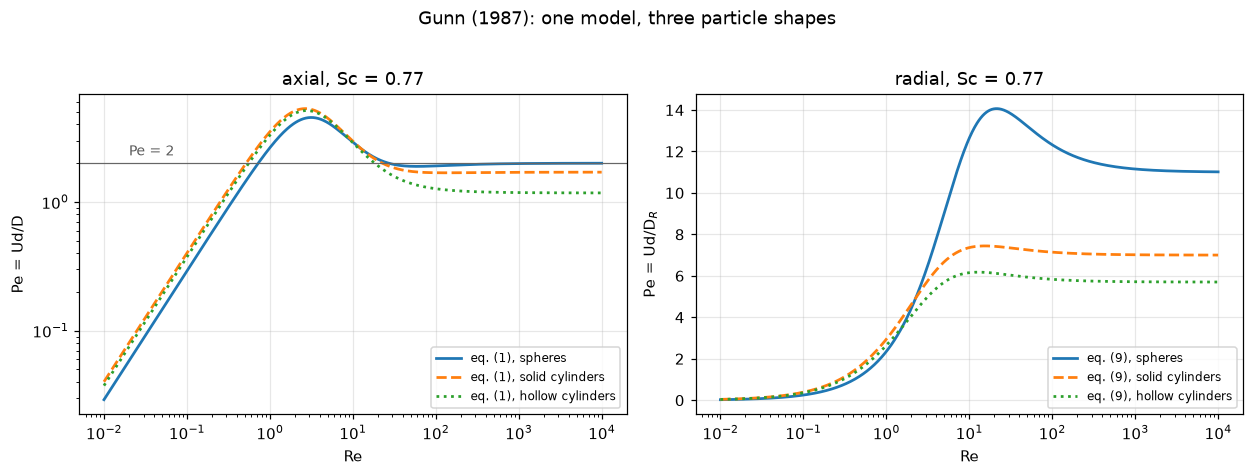
Pe_f (eqs 10-12) at Re -> 0 and Re -> infinity, in closed form:
  spheres            40.00  ->   11.00
  solid cylinders    11.00  ->    7.00
  hollow cylinders    9.00  ->    5.70

D_axial / D_radial in the high-Re limit, spheres: Pe_f(inf) / Pe_ax(inf) = 5.500
  (eq. (9) and eq. (1) evaluated at Re = 1e6 give 5.5001)

and the same beds carry two tortuosities: 1.4 in eq. (3) against 1.2 in eq. (10), a difference of +17%,
which the paper describes only as differing 'by small amounts'. Both are used here, each in its own direction; swapping them is a break-table row.
The textbook ratio of axial to radial dispersion at high flow, “5 to 6”, falls out of two correlations fitted to different experiments, neither of which was asked for that ratio: the closed-form limit above is the ratio of eq. (10)’s high-Reynolds value to the sphere limit of eq. (1).
2. What the wall channel costs, and what radial dispersion puts back
Gunn’s eqs (7) and (8) argue that the high-porosity layer within \(0.5d\) of the wall does not carry a significantly faster interstitial velocity, because the superficial ratio Price measured is mostly porosity. The argument is qualitative, “suggesting that there may be no significant differences”. A 2-D bed turns it into a number, and it needs the radial coefficient to do it, because radial dispersion is what erodes a wall channel once it exists.
Three velocity profiles are run at the operating point printed in the implementation section: uniform; Gunn’s corrected interstitial ratio; and the ratio you get by reading Price’s 1.65 as interstitial, which is the mistake his eq. (8) exists to prevent. Each is run with the radial coefficient eq. (9) gives, and again with radial dispersion switched off, so the two effects separate. The measure is the mixing-cup concentration on the outlet face, weighted by the local flux. The annulus is resolved by the radial grid: its edge is a cell face on every grid below, and the radial grid is refined until its effect on the answer is measured.
U_RATIO_GUNN = CS["wall_velocity_ratio"]
R165 = G["superficial_velocity_ratio_price"]
NO_RADIAL = 1e-12               # D_R -> 0: the columns decouple
WALL_GRID = (800, 160)          # n_z, n_r for every wall-channel number


@lru_cache(maxsize=None)
def wall_cup(ratio_w, d_r, n_z=WALL_GRID[0], n_r=WALL_GRID[1], extent=None,
             local_inlet=False):
    """Mixing-cup outlet concentration of the bed with a wall annulus."""
    ext = G["wall_region_extent_diameters"] if extent is None else extent
    if ratio_w == 1.0 and extent is not None:        # a uniform bed has no annulus
        return wall_cup(1.0, d_r, n_z, n_r, None, local_inlet)
    b = bed(D_R=d_r, n_z=n_z, n_r=n_r, wall_ratio=ratio_w, wall_extent=ext,
            local_inlet=local_inlet).solve()
    return b.cup()


def wall_cost(ratio_w, d_r, **kw):
    """Extra unconverted reactant against the uniform bed run with the same settings."""
    return wall_cup(ratio_w, d_r, **kw) / wall_cup(1.0, d_r, **kw) - 1.0


runs = []
for label, ratio_w in [("uniform", 1.0), ("Gunn eq. (8) interstitial ratio", U_RATIO_GUNN),
                       ("1.65 read as interstitial", R165)]:
    for rad_label, d_r in [("eq. (9)", DR_OP), ("none", NO_RADIAL)]:
        runs.append(dict(profile=label, radial=rad_label, U_w_over_U_b=ratio_w,
                         c_out=wall_cup(ratio_w, d_r), unconverted_vs_uniform=wall_cost(ratio_w, d_r)))
runs = pd.DataFrame(runs)
print(f"grid n_z x n_r = {WALL_GRID[0]} x {WALL_GRID[1]}")
print(runs.to_string(index=False, float_format=lambda v: f"{v:.6f}"))

NAIVE_WITH = wall_cost(R165, DR_OP)
NAIVE_WITHOUT = wall_cost(R165, NO_RADIAL)
GUNN_WITH, GUNN_WITHOUT = wall_cost(U_RATIO_GUNN, DR_OP), wall_cost(U_RATIO_GUNN, NO_RADIAL)
HEAL = 1 - NAIVE_WITH / NAIVE_WITHOUT
# The Robin inlet is written with the AREA-MEAN velocity U (see the bc table).
# Writing the same balance with the local u(r) is the other defensible reading;
# it is measured rather than argued about, and it is a break-table row.
NAIVE_WITH_LOCAL = wall_cost(R165, DR_OP, local_inlet=True)
NAIVE_WITHOUT_LOCAL = wall_cost(R165, NO_RADIAL, local_inlet=True)
LOCAL_MOVE = abs(dev(NAIVE_WITH_LOCAL, NAIVE_WITH))

# the radial grid: n_r refined at n_z = 800, successive differences only
WALL_NR = (20, 40, 80, 160)
wall_lad = observed_orders(lambda n: wall_cost(R165, DR_OP, n_r=n), WALL_NR)
WALL_R_ORDERS = np.asarray(wall_lad["orders"])
WALL_EXTRAP = float(wall_lad["extrapolated"])
WALL_GRID_ERR = NAIVE_WITH / WALL_EXTRAP - 1
print(f"\nradial grid, 1.65 with eq. (9)'s D_R, n_z = {WALL_GRID[0]}:")
for n, v in zip(WALL_NR, wall_lad["values"]):
    print(f"  n_r = {n:4d}   cost {v:+.6%}")
print(f"  observed orders {', '.join(f'{o:.3f}' for o in WALL_R_ORDERS)}; Richardson "
      f"estimate {WALL_EXTRAP:+.4%}, so n_r = {WALL_GRID[1]} is {WALL_GRID_ERR:+.2%} of it")

display(Markdown(rf"""
**Reading Price's {R165} as an interstitial ratio raises the unconverted reactant
leaving this bed by {NAIVE_WITHOUT:+.2%} with no radial mixing, and by
{NAIVE_WITH:+.2%} once eq. (9)'s radial coefficient is switched on**, so radial
dispersion erodes {HEAL:.0%} of the channel over this bed length. Gunn's corrected
ratio, {U_RATIO_GUNN:.4f}, moves the outlet by {GUNN_WITH:+.4%} with radial
dispersion and {GUNN_WITHOUT:+.4%} without it. **The whole of the effect is in the
difference between 1.65 and 1.02**, which is what eq. (8) is for; at Gunn's
corrected ratio the wall region is not worth putting in a model at all.

The radial grid matters here and is measured: refining $n_r$ from {WALL_NR[0]} to
{WALL_NR[-1]} converges at observed orders {WALL_R_ORDERS.min():.2f} to
{WALL_R_ORDERS.max():.2f}, and the value on {WALL_GRID[1]} radial cells is
{WALL_GRID_ERR:+.2%} of its Richardson estimate {WALL_EXTRAP:+.3%}. On
{WALL_NR[1]} radial cells the same number is {wall_lad['values'][1]:+.3%}, a grid
value.

Three honest limits on that number. It is **one operating point**: the erosion
fraction depends on $L/d$, on $d_t/d$ and on the Damköhler group, and none of the
three is printed anywhere in the paper. The wall annulus here is a *step*, not
the smooth porosity profile a real bed has: the step is what the paper's own
"wall region of extent {G['wall_region_extent_diameters']}$d$" describes, and no
more; widening it is a break-table row. And the Danckwerts inlet is written with
the **area-mean** velocity, $Uc - D\,\partial c/\partial z = Uc_0$, rather than with
the local $u(r)$: writing the same balance locally gives {NAIVE_WITH_LOCAL:+.3%}
instead of {NAIVE_WITH:+.3%} and {NAIVE_WITHOUT_LOCAL:+.3%} instead of
{NAIVE_WITHOUT:+.3%}, so the erosion fraction moves from {HEAL:.1%} to
{1 - NAIVE_WITH_LOCAL / NAIVE_WITHOUT_LOCAL:.1%}. The choice is a modelling
convention the paper does not fix, it changes the answer by
{LOCAL_MOVE:.1%} of itself, and no conclusion here depends on it.
"""))
grid n_z x n_r = 800 x 160
profile radial U_w_over_U_b c_out unconverted_vs_uniform
uniform eq. (9) 1.000000 0.136736 0.000000
uniform none 1.000000 0.136736 0.000000
Gunn eq. (8) interstitial ratio eq. (9) 1.017500 0.136737 0.000009
Gunn eq. (8) interstitial ratio none 1.017500 0.136743 0.000052
1.65 read as interstitial eq. (9) 1.650000 0.138298 0.011424
1.65 read as interstitial none 1.650000 0.144204 0.054614
radial grid, 1.65 with eq. (9)'s D_R, n_z = 800:
n_r = 20 cost +1.202514%
n_r = 40 cost +1.156978%
n_r = 80 cost +1.145314%
n_r = 160 cost +1.142359%
observed orders 1.965, 1.981; Richardson estimate +1.1414%, so n_r = 160 is +0.09% of itReading Price’s 1.65 as an interstitial ratio raises the unconverted reactant leaving this bed by +5.46% with no radial mixing, and by +1.14% once eq. (9)’s radial coefficient is switched on, so radial dispersion erodes 79% of the channel over this bed length. Gunn’s corrected ratio, 1.0175, moves the outlet by +0.0009% with radial dispersion and +0.0052% without it. The whole of the effect is in the difference between 1.65 and 1.02, which is what eq. (8) is for; at Gunn’s corrected ratio the wall region is not worth putting in a model at all.
The radial grid matters here and is measured: refining \(n_r\) from 20 to 160 converges at observed orders 1.96 to 1.98, and the value on 160 radial cells is +0.09% of its Richardson estimate +1.141%. On 40 radial cells the same number is +1.157%, a grid value.
Three honest limits on that number. It is one operating point: the erosion fraction depends on \(L/d\), on \(d_t/d\) and on the Damköhler group, and none of the three is printed anywhere in the paper. The wall annulus here is a step, not the smooth porosity profile a real bed has: the step is what the paper’s own “wall region of extent 0.5\(d\)” describes, and no more; widening it is a break-table row. And the Danckwerts inlet is written with the area-mean velocity, \(Uc - D\,\partial c/\partial z = Uc_0\), rather than with the local \(u(r)\): writing the same balance locally gives +1.130% instead of +1.142% and +5.482% instead of +5.461%, so the erosion fraction moves from 79.1% to 79.4%. The choice is a modelling convention the paper does not fix, it changes the answer by 1.0% of itself, and no conclusion here depends on it.
Validation
Ranked as the builder brief ranks them, best first. Route 1 is available here (the paper contains a worked example with every input printed), and so is route 2, several times over. The figure route is used once, through a dataset another page already extracted and audited.
V1. A worked example with printed intermediates: eq. (8)
\(u_w/u_b = 1.65\), \(e = 0.37\), \(\bar e_w = 0.6\), all printed, and the answer \(U_w/U_b = 1.02\) printed too.
WALL_DEV = CS["wall_velocity_ratio_rel_dev"]
eps_w_mean = 0.5 * (G["voidage_wall_range_min"] + G["voidage_wall_range_max"])
U_ratio_at = lambda e_w: G["superficial_velocity_ratio_price"] * G["voidage_bulk_spheres"] / e_w
print(f"eq. (8): {G['superficial_velocity_ratio_price']} x "
      f"{G['voidage_bulk_spheres']} / {G['voidage_wall_region']} = {U_RATIO_GUNN:.5f}")
print(f"  printed {G['interstitial_velocity_ratio_result']}  ->  {WALL_DEV:+.3%}, "
      "inside half a unit of the printed second decimal")
print(f"  the paper says e_w is LESS than the mean of {G['voidage_wall_range_min']} "
      f"and {G['voidage_wall_range_max']}; AT that mean ({eps_w_mean}) eq. (8) gives "
      f"{U_ratio_at(eps_w_mean):.4f}, a wall SLOWER than the bulk,")
print("  which is why the paper picks a value below it")
print(f"  at e_w = 0.5 it gives {U_ratio_at(0.5):.4f} "
      f"({dev(U_ratio_at(0.5), U_RATIO_GUNN):+.1%}), so the check has power "
      "against a mis-read wall porosity")
eq. (8): 1.65 x 0.37 / 0.6 = 1.01750
printed 1.02 -> -0.245%, inside half a unit of the printed second decimal
the paper says e_w is LESS than the mean of 0.37 and 1.0; AT that mean (0.685) eq. (8) gives 0.8912, a wall SLOWER than the bulk,
which is why the paper picks a value below it
at e_w = 0.5 it gives 1.2210 (+20.0%), so the check has power against a mis-read wall porosityV2. Internal identities
Four, none of which needs a figure or a solver.
(a) The high-Re limit, by expansion and then by direct evaluation, done above for all three shapes.
(b) The low-ReSc limit against Edwards and Richardson’s independently measured tortuosity factor. As \(\mathrm{Re\,Sc}\to0\), eq. (1) gives \(D/(Ud)\to\varepsilon/(\tau\mathrm{Re\,Sc})\), i.e. \(\mathrm{Pe}\to\tau\mathrm{Re\,Sc}/\varepsilon\). E&R’s eq. (18) gives \(\mathrm{Pe}\to\mathrm{Re}/a\) with \(a\) its printed molecular coefficient, which is \(\gamma\varepsilon/\mathrm{Sc}\), so their limit is \(\mathrm{Re\,Sc}/(\gamma\varepsilon)\). The same expression, with \(\tau\) where they have \(1/\gamma\) and \(\varepsilon\) in the same place: both a check on two transcriptions made from different papers and a corroboration that the two \(\mathrm{Re}\)’s and \(\mathrm{Pe}\)’s mean the same quantities.
(c) The same model as two different papers print it. Gunn’s 1993 note gives eq. (42) with \(\Gamma = 4(1-\varepsilon)\alpha_1^2/\varepsilon\). Substituting \(\Gamma\) turns it into eq. (1) term by term. The two forms are transcribed from different documents, so agreement is evidence about the reading; it says nothing about whether either reading is right. A difference in one reading (an \(\alpha_1\) read differently in one of them) is a break row.
(d) The closed form solves the equation. Eq. (17) put back into eq. (16) and into the Danckwerts inlet, algebraically: \(c = C e^{-\lambda x}\) solves eq. (16) iff \(D\lambda^2 + U\lambda - k = 0\), and satisfies the inlet iff \(C(U + D\lambda) = Uc_0\). Both are evaluated with \(\lambda\) and \(C\) as eq. (17) prints them.
TAU_G = G["tau_axial_spheres"]
print("low-Re asymptote Pe/Re, from each paper's own printed constants")
print(f"  Gunn eq. (1):   tau Sc / eps  = {TAU_G} x {SC} / {EPS} = {TAU_G * SC / EPS:.4f}")
print(f"  E&R  eq. (18):  1 / {E['eq18_molecular_coefficient']}            = "
      f"{1 / E['eq18_molecular_coefficient']:.4f}")
print(f"  ratio {CS['low_re_slope_gunn_over_er']:.4f}, i.e. "
      f"{CS['low_re_slope_gunn_over_er'] - 1:+.1%}")
print(f"  the two tortuosities: Gunn tau = {TAU_G} -> 1/tau = {1 / TAU_G:.4f} against "
      f"E&R's separately measured gamma = {E['tortuosity_factor_gamma']}  "
      f"({CS['tau_inverse_vs_er_gamma_rel_dev']:+.2%})")
print(f"  Schmidt group for argon-air: Gunn {SC}, E&R {E['schmidt_number_used_in_eq18']} "
      f"({dev(SC, E['schmidt_number_used_in_eq18']):+.1%}), printed as they stand")
print("  Both papers put eps in the same place in this limit, and both assert Pe -> 2")
print("  at high Re. As a further leg: if E&R's markers had to be divided by eps to")
print(f"  reach Gunn's axes they would peak at Pe = {Pe_d.max() / EPS:.2f} (the largest "
      f"marker, Re = {Re_d[np.argmax(Pe_d)]:.2f}, divided by eps), where eq. (1) peaks")
print(f"  at {CS['eq1_peclet_maximum']:.2f} (section V3).")

print(f"\n(c) eq. (1) [1987] against eq. (42) [1993], both evaluated with expm1, at Sc = "
      f"{SC} and {SC_LIQ:g} over 2001 Re: max relative difference below 1e-9 "
      f"(here {CS['eq1_vs_eq42_identity']:.1e})")
print("    the SAME expression written with exp(x) - 1 instead of expm1(x) differs by "
      f"more than 1e-7 (here {CS['expm1_vs_naive_exp_worst']:.1e}) at Sc = {SC_LIQ:g}:")
print("    the identity is algebraic, the arithmetic is not")


def lam_eq17(U, D, k, sign=-1.0):
    """lambda as eq. (17) prints it: sqrt(U^2/4D^2 + k/D) - U/2D (sign -1)."""
    return np.sqrt(U ** 2 / (4 * D ** 2) + k / D) + sign * U / (2 * D)


def eq17_identities(U, D, k, sign=-1.0):
    """Worst relative residual of eq. (17) in eq. (16) and in the Danckwerts inlet."""
    lam = lam_eq17(U, D, k, sign)
    C = U / (U + D * lam)                     # eq. (17)'s prefactor, c0 = 1
    return max(abs(D * lam ** 2 + U * lam - k) / k, abs(C * (U + D * lam) - U) / U)


EQ17_ID = max(eq17_identities(1.0, D_OP, k) for k in (K_OP, 1e-4, 1.0))
print(f"\n(d) eq. (17) in eq. (16) and in the Danckwerts inlet, at kL/U = 0.01, 2 and 100: "
      f"worst relative residual below 1e-10 (here {EQ17_ID:.1e})")
low-Re asymptote Pe/Re, from each paper's own printed constants
Gunn eq. (1): tau Sc / eps = 1.4 x 0.77 / 0.37 = 2.9135
E&R eq. (18): 1 / 0.38 = 2.6316
ratio 1.1071, i.e. +10.7%
the two tortuosities: Gunn tau = 1.4 -> 1/tau = 0.7143 against E&R's separately measured gamma = 0.73 (-2.15%)
Schmidt group for argon-air: Gunn 0.77, E&R 0.72 (+6.9%), printed as they stand
Both papers put eps in the same place in this limit, and both assert Pe -> 2
at high Re. As a further leg: if E&R's markers had to be divided by eps to
reach Gunn's axes they would peak at Pe = 11.24 (the largest marker, Re = 4.37, divided by eps), where eq. (1) peaks
at 4.53 (section V3).
(c) eq. (1) [1987] against eq. (42) [1993], both evaluated with expm1, at Sc = 0.77 and 800 over 2001 Re: max relative difference below 1e-9 (here 1.2e-10)
the SAME expression written with exp(x) - 1 instead of expm1(x) differs by more than 1e-7 (here 1.7e-06) at Sc = 800:
the identity is algebraic, the arithmetic is not
(d) eq. (17) in eq. (16) and in the Danckwerts inlet, at kL/U = 0.01, 2 and 100: worst relative residual below 1e-10 (here 1.3e-12)V3. Numbers the paper states in words
Seven, each of which can fail on a single mis-read digit, and none of which involves reading a figure. Each is compared with the precision of the phrase that states it, counted in half-units of its last printed digit; the unit is printed beside each, and for the two plateaus of \(p\) it is the second decimal to which \(p\)’s own constants are printed.
p_inf_sph = G["p_offset"] + G["p_amplitude_spheres"]
p_lo = float(p_of_Re(G["reynolds_p_lower_plateau"], G))
p_hi = float(p_of_Re(G["reynolds_p_upper_plateau"], G))
p_mid = float(p_of_Re(G["reynolds_p_transition_end"], G))
PHRASES = [  # (quantity, computed, printed, unit of the last printed digit, phrase)
    ("Pe at Re = 1000, Sc = 0.77", CS["pe_at_Re_1000"], G["peclet_high_re_asymptote"], 1.0,
     "'Pe approaches the widely quoted value of 2'"),
    ("p at Re = 1, against its Re -> 0 plateau", p_lo, G["p_offset"], 0.01,
     "'constant values for p below Re = 1'"),
    ("p at Re = 1000, against its Re -> inf plateau", p_hi, p_inf_sph, 0.01,
     "'constant values for p ... above 1000'"),
    ("max liquid/gas ratio of D/(Ud)", CS["liquid_gas_max_ratio"],
     G["liquid_gas_max_factor"], 1.0, "'a maximum difference of a factor of 10'"),
    ("Re at that maximum", CS["liquid_gas_max_reynolds"], G["liquid_gas_max_reynolds"], 1.0,
     "'at Re ~ 3'"),
    ("Re where liquid D/(Ud) overtakes gas", CS["liquid_gas_crossover_reynolds"],
     G["liquid_gas_range_min"], 0.1, "'within the range of 0.2 < Re < 300'"),
    ("mean of Table 1's entries", T1["table1_mean"],
     G["intraparticle_diffusivity_fraction"], 0.01, "'about 10 % of molecular (Table 1)'"),
]
chk = pd.DataFrame(PHRASES, columns=["quantity", "computed", "printed", "unit", "as printed"])
chk["dev"] = dev(chk.computed, chk.printed)
chk["half_units"] = (chk.computed - chk.printed).abs() / (chk.unit / 2)
print(chk.drop(columns="as printed").to_string(index=False, float_format=lambda v: f"{v:.4f}"))
for q, phrase in zip(chk.quantity, chk["as printed"]):
    print(f"  {q:46s} {phrase}")
HALF_UNITS = chk.half_units.to_numpy()
N_INSIDE = int(np.sum(HALF_UNITS <= 1.0))
FACTOR10_ONE_DIGIT = abs(CS["liquid_gas_max_ratio"] - G["liquid_gas_max_factor"]) / 5.0
print(f"\nand the shape of p, which the paper describes rather than tabulates:")
print(f"  p(1) = {p_lo:.5f}, p(200) = {p_mid:.5f}, p(1000) = {p_hi:.5f}, "
      f"p(inf) = {p_inf_sph:.2f}")
print(f"  -> {CS['fraction_of_p_excursion_1_to_200']:.1%} of p's total excursion happens "
      "between Re = 1 and 200, which is what")
print("     'the major change in p taking place from Re = 1 to 200' asserts")

display(Markdown(rf"""
**{N_INSIDE} of the {len(chk)} stated numbers lie within half a unit of their last
printed digit; the deviations run from {chk.dev.abs().min():.1%} to
{chk.dev.abs().max():.1%}.** The two that do not:

- $p(1000)$ sits {abs(CS['p_at_Re_1000_rel_dev']):.1%} below the high-Reynolds
  plateau, {chk.half_units[2]:.2f} half-units of the second decimal to which the
  paper prints $p$'s constants: "constant above 1000" holds to
  {abs(CS['p_at_Re_1000_rel_dev']):.1%}, not to the printed digits.
- the liquid/gas maximum, {CS['liquid_gas_max_ratio']:.2f}, is
  {chk.half_units[3]:.2f} half-units from "a factor of 10" read as an integer, and
  {FACTOR10_ONE_DIGIT:.2f} half-units if the 10 carries one significant figure.

None of these phrases is printed to more than two figures, so none could have been
checked more tightly; what they *can* do, and the break table shows they do, is
fail on a mis-read digit.

The one statement that does *not* survive is the **upper** end of
"0.2 < Re < 300", and it fails for a structural reason rather than a numerical
one: it is not a crossing at all. A root scan of the liquid/gas ratio minus one
over Re = 0.001 to 10⁶ finds {CS['liquid_gas_crossings']} sign change, at
Re = {CS['liquid_gas_crossover_reynolds']:.3f}; above it the ratio decays towards 1
from above and is still **{CS['liquid_gas_ratio_at_Re_300']:.3f}** at
Re = {G['liquid_gas_range_max']:.0f} and {CS['liquid_gas_ratio_at_Re_1000']:.3f} at
Re = 1000. Read as "the range over which the difference matters", 300 is a
judgement; read as a crossing it is wrong.

The Péclet limit is the interesting near-miss. Eq. (1) gives
{CS['pe_at_Re_1000']:.4f} at Re = 1000, {abs(dev(CS['pe_at_Re_1000'], 2.0)):.2%}
below 2, and does not come within 5e-4 of 2 until
Re = {CS['reynolds_pe_within_5e-4_of_2']:.3g} (root-found). On the way it is not
monotone: for argon in air at $\varepsilon$ = {EPS}, eq. (1) has a Péclet maximum of {CS['eq1_peclet_maximum']:.4f} at
Re = {CS['eq1_peclet_maximum_reynolds']:.4f} and a minimum of
{CS['eq1_peclet_minimum']:.4f} at Re = {CS['eq1_peclet_minimum_reynolds']:.2f}, the
two roots of the analytic derivative on Re = 0.001 to 10⁵. "Approaching 1000" is
the right way to say it, and a page that reported "2.000" here would be reporting
the asymptote rather than the equation.
"""))
quantity computed printed unit dev half_units
Pe at Re = 1000, Sc = 0.77 1.9862 2.0000 1.0000 -0.0069 0.0275
p at Re = 1, against its Re -> 0 plateau 0.1700 0.1700 0.0100 0.0000 0.0000
p at Re = 1000, against its Re -> inf plateau 0.4922 0.5000 0.0100 -0.0157 1.5651
max liquid/gas ratio of D/(Ud) 10.8909 10.0000 1.0000 0.0891 1.7819
Re at that maximum 3.1662 3.0000 1.0000 0.0554 0.3325
Re where liquid D/(Ud) overtakes gas 0.1771 0.2000 0.1000 -0.1143 0.4571
mean of Table 1's entries 0.0970 0.1000 0.0100 -0.0300 0.6000
Pe at Re = 1000, Sc = 0.77 'Pe approaches the widely quoted value of 2'
p at Re = 1, against its Re -> 0 plateau 'constant values for p below Re = 1'
p at Re = 1000, against its Re -> inf plateau 'constant values for p ... above 1000'
max liquid/gas ratio of D/(Ud) 'a maximum difference of a factor of 10'
Re at that maximum 'at Re ~ 3'
Re where liquid D/(Ud) overtakes gas 'within the range of 0.2 < Re < 300'
mean of Table 1's entries 'about 10 % of molecular (Table 1)'
and the shape of p, which the paper describes rather than tabulates:
p(1) = 0.17000, p(200) = 0.46268, p(1000) = 0.49217, p(inf) = 0.50
-> 88.7% of p's total excursion happens between Re = 1 and 200, which is what
'the major change in p taking place from Re = 1 to 200' asserts5 of the 7 stated numbers lie within half a unit of their last printed digit; the deviations run from 0.0% to 11.4%. The two that do not:
- \(p(1000)\) sits 1.6% below the high-Reynolds plateau, 1.57 half-units of the second decimal to which the paper prints \(p\)’s constants: “constant above 1000” holds to 1.6%, not to the printed digits.
- the liquid/gas maximum, 10.89, is 1.78 half-units from “a factor of 10” read as an integer, and 0.18 half-units if the 10 carries one significant figure.
None of these phrases is printed to more than two figures, so none could have been checked more tightly; what they can do, and the break table shows they do, is fail on a mis-read digit.
The one statement that does not survive is the upper end of “0.2 < Re < 300”, and it fails for a structural reason rather than a numerical one: it is not a crossing at all. A root scan of the liquid/gas ratio minus one over Re = 0.001 to 10⁶ finds 1 sign change, at Re = 0.177; above it the ratio decays towards 1 from above and is still 1.084 at Re = 300 and 1.025 at Re = 1000. Read as “the range over which the difference matters”, 300 is a judgement; read as a crossing it is wrong.
The Péclet limit is the interesting near-miss. Eq. (1) gives 1.9862 at Re = 1000, 0.69% below 2, and does not come within 5e-4 of 2 until Re = 2.85e+04 (root-found). On the way it is not monotone: for argon in air at \(\varepsilon\) = 0.37, eq. (1) has a Péclet maximum of 4.5274 at Re = 3.1513 and a minimum of 1.8886 at Re = 59.66, the two roots of the analytic derivative on Re = 0.001 to 10⁵. “Approaching 1000” is the right way to say it, and a page that reported “2.000” here would be reporting the asymptote rather than the equation.
The derivative those extrema are roots of is checked against an independent one: mpmath differentiates eq. (1) numerically in 40-digit arithmetic, which shares only the transcription with dD_over_Ud_dRe.
mp.mp.dps = 40
_A1 = mp.besseljzero(0, 1)


def D_over_Ud_mp(Re, Sc, shape="spheres", alpha1=None):
    """Eq. (1) in mpmath arithmetic, an independent reference for its derivative."""
    a1 = _A1 if alpha1 is None else mp.mpf(alpha1)
    tau = G[SHAPES[shape][1]]
    p = G["p_offset"] + G[SHAPES[shape][0]] * mp.e ** (-G["p_reynolds_scale"] / Re)
    A = Re * Sc / (4 * a1 ** 2 * (1 - EPS))
    return (A * (1 - p) ** 2 + A ** 2 * p * (1 - p) ** 3 * mp.expm1(-1 / (A * p * (1 - p)))
            + EPS / (tau * Re * Sc))


def derivative_check(alpha1_analytic=ALPHA1):
    """Worst |analytic - mpmath| derivative, scaled by D/(Ud)/Re, over shapes, Sc and Re."""
    worst = 0.0
    for s in SHAPES:
        for sc_ in (SC, SC_LIQ):
            for R in np.logspace(-3, 5, 17):
                ref = mp.diff(lambda x: D_over_Ud_mp(x, sc_, s), mp.mpf(R))
                an = float(dD_over_Ud_dRe(R, sc_, G, EPS, shape=s, alpha1=alpha1_analytic))
                worst = max(worst, abs(an - float(ref)) / (float(D_over_Ud_mp(mp.mpf(R), sc_, s)) / R))
    return worst


DERIV_CHECK = derivative_check()
print(f"analytic derivative of eq. (1) against mpmath, three shapes, Sc = {SC} and "
      f"{SC_LIQ:g}, Re = 0.001 to 1e5:")
print(f"  worst difference, in units of D/(Ud)/Re, below 1e-7 (here {DERIV_CHECK:.1e})")
analytic derivative of eq. (1) against mpmath, three shapes, Sc = 0.77 and 800, Re = 0.001 to 1e5:
worst difference, in units of D/(Ud)/Re, below 1e-7 (here 1.3e-09)V4. Against measurement: eq. (1) on the markers A2.5 digitised
Gunn’s Figure 1 plots Edwards and Richardson’s gas-phase points as one of its four series, and asserts that eq. (1) with eq. (3) describes them. A2.5 has those measurements as a CSV, so the assertion is testable here without touching a figure. Three things have to be said before the number is read.
Are these markers inside Gunn’s fit set? The printed evidence says probably not.
- Gunn 1987, journal page 365: “values of the probability \(p\) were estimated from dispersion experiments in which the effect of molecular diffusion was very small and given as a table showing the change with Reynolds number.”
- Gunn 1993, journal page 335, saying what that criterion meant: “when \(\mathrm{Re\,Sc}\gg 1\), measurements of dispersion are not affected by molecular diffusion and therefore experimental measurements of liquid-phase dispersion may be used to find the dependence of \(p\) upon the Reynolds number and this has been carried out for beds of spheres, solid cylinders and hollow cylinders [2, 5]. The experimental results for both gas-phase and liquid-phase dispersion may then be used to compare the predictions of eqn. (42) with experiment.” Refs [2] and [5] are Gunn 1969 and Gunn 1987; Edwards and Richardson are [7], cited separately as one of the two gas-phase sets Figure 1 compares against.
- These markers fail that criterion. They are gas phase at \(\mathrm{Sc} = 0.77\); the cell below prints the \(\mathrm{Re\,Sc}\) distribution, and it is nowhere near \(\gg 1\).
- Where the 1987 paper does name a fit set, it is not this one. Eqs (4) and (5) are “based upon the experimental results of England and Gunn (1970), for the dispersion of argon in beds of solid and hollow cylinders” (page 366); eq. (3) is attributed to nothing. The sentence that introduces all three (“a study of the experimental results for dispersion in beds of spheres, and in beds of cylinders shows that the dependence of \(p\) upon Reynolds number may be expressed by the following equations”) names no dataset. Meanwhile the paper’s own sentence about these points is the language of comparison: “the experimental estimates of Edwards and Richardson for (1968) the dispersion of argon in air are well supported by eq. (1)” (page 366).
So the honest label is a comparison that is probably out of sample but not provably held out: closer to a test of eq. (1) than to a fit residual, and much further from circular than A2.5’s own headline, where both constants were fitted to exactly these markers and nothing else. Nothing printed says these points were held out either, so the page does not call the comparison a validation.
The porosity is not printed, and it is a large lever on the answer. The study below runs the comparison at \(\varepsilon\) = 0.34, 0.37 and 0.40, and finds the porosity the markers prefer.
One shape, one gas pair, and a Reynolds range that stops at 50 where \(p(\mathrm{Re})\) is still climbing. The study prints how much of \(p\)’s excursion the dataset spans and what replacing \(p(\mathrm{Re})\) by a constant costs, with the standard error of that cost.
Minimisations of a mean absolute deviation are not smooth, so each is done the same way: a scan of the whole window, then a bounded minimisation inside the two scan cells around the lowest scan point, accepted only if it is not above the scan minimum and the scan minimum is not on the window’s edge. The number of local minima on the scan is printed, because one of these functions has two.
def _scan_min(f_vec, lo, hi, n):
    """Scan f on n points of [lo, hi], then refine inside the bracketing scan cells."""
    xs = np.linspace(lo, hi, n)
    fs = np.asarray(f_vec(xs), float)
    i = int(np.argmin(fs))
    if i in (0, n - 1):
        raise ValueError(f"scan minimum on the edge of [{lo:g}, {hi:g}]")
    r = minimize_scalar(lambda x: float(f_vec(np.array([x]))[0]),
                        bounds=(xs[i - 1], xs[i + 1]), method="bounded",
                        options={"xatol": 1e-12})
    if r.fun > fs[i] + 1e-15:
        raise ValueError("refinement above the scan minimum")
    n_local = int(np.sum((fs[1:-1] < fs[:-2]) & (fs[1:-1] < fs[2:])))
    return float(r.x), float(r.fun), n_local


P_WINDOW, EPS_WINDOW = (0.001, 0.95), (0.28, 0.58)


def data_study(G, eps=EPS, eq1=None, E=E, re=Re_d, pe=Pe_d, px_per_decade=None):
    """Eq. (1) against the markers, the nulls, the porosity and the systematics."""
    eq1 = dict(eq1 or {})
    sc = G["schmidt_argon_air"]
    n = len(pe)
    px = PX_PER_DECADE_PE if px_per_decade is None else px_per_decade
    mad = lambda d: float(np.mean(np.abs(d)))
    model = lambda e, R=re, **k: Pe_axial(R, sc, G, e, **{**eq1, **k})
    out, refused = {}, []
    d = dev(model(eps), pe)
    out["eq1_vs_fig9_mean_abs_dev"] = mad(d)
    out["eq1_vs_fig9_bias"] = float(d.mean())
    out["eq1_vs_fig9_bias_over_se"] = float(d.mean() / (d.std(ddof=1) / np.sqrt(n)))
    resc = re * sc
    out["resc_min"], out["resc_max"] = float(resc.min()), float(resc.max())
    out["resc_median"] = float(np.median(resc))
    out["n_resc_below_1"] = int(np.sum(resc < 1.0))
    out["n_resc_below_10"] = int(np.sum(resc < 10.0))
    # E&R's own eq. (18) and its uncorrected eq. (15), recomputed from the same file
    a, b, c = (E["eq18_molecular_coefficient"], E["eq18_eddy_coefficient"],
               E["eq18_correction_coefficient"])
    d18 = dev(1.0 / (a / re + b / (1.0 + c / re)), pe)
    out["eq18_vs_fig9_mean_abs_dev_recomputed"] = mad(d18)
    out["eq18_vs_fig9_bias_recomputed"] = float(d18.mean())
    out["null_eq15_mean_abs_dev"] = mad(dev(1.0 / (a / re + b), pe))
    # E&R's maximum in closed form: d/dRe [a/Re + b/(1 + c/Re)] = 0
    re18 = c / (np.sqrt(b * c / a) - 1.0)
    out["eq18_re_at_pe_max_recomputed"] = float(re18)
    out["eq18_pe_max_recomputed"] = float(1.0 / (a / re18 + b / (1.0 + c / re18)))
    # nulls: p frozen at a printed plateau, and p a FREE constant (the strongest)
    p_off, p_inf = G["p_offset"], G["p_offset"] + G["p_amplitude_spheres"]
    out["null_p_frozen_low_mean_abs_dev"] = mad(dev(model(eps, p=np.full(n, p_off)), pe))
    out["null_p_frozen_high_mean_abs_dev"] = mad(dev(model(eps, p=np.full(n, p_inf)), pe))
    mad_p = lambda pp, e: np.mean(np.abs(dev(model(e, p=np.asarray(pp)[:, None]
                                                  * np.ones(n)[None, :]), pe)), axis=1)
    try:
        pf, nf, nloc = _scan_min(lambda pp: mad_p(pp, eps), *P_WINDOW, 1901)
        dn = dev(model(eps, p=np.full(n, pf)), pe)
        diff = np.abs(dn) - np.abs(d)
        out.update({"null_free_constant_p_value": pf, "null_free_constant_p_mean_abs_dev": nf,
                    "null_free_constant_p_local_minima": nloc,
                    "p_cost_vs_free_constant": float(diff.mean()),
                    "p_cost_vs_free_constant_over_se": float(diff.mean()
                                                            / (diff.std(ddof=1) / np.sqrt(n))),
                    "null_free_constant_p_sensitivity": float(
                        max(mad_p([0.9 * pf, 1.1 * pf], eps)) - nf)})
    except ValueError as exc:
        refused.append(f"free p: {exc}")
        for k in ("null_free_constant_p_value", "null_free_constant_p_mean_abs_dev",
                  "null_free_constant_p_local_minima", "p_cost_vs_free_constant",
                  "p_cost_vs_free_constant_over_se", "null_free_constant_p_sensitivity"):
            out[k] = np.nan
    # the porosity: two fixed readings, and the porosity each model prefers
    mad_eps = lambda es: np.array([mad(dev(model(e), pe)) for e in es])
    out["eq1_vs_fig9_mad_eps_034"], out["eq1_vs_fig9_mad_eps_040"] = mad_eps([0.34, 0.40])
    try:
        eb, mb, nl = _scan_min(mad_eps, *EPS_WINDOW, 601)
        # a free constant p at every porosity: a 2-D scan, then a nested refinement
        es, ps = np.linspace(*EPS_WINDOW, 121), np.linspace(*P_WINDOW, 476)
        surf = np.array([mad_p(ps, e) for e in es])
        i, j = np.unravel_index(np.argmin(surf), surf.shape)
        if i in (0, len(es) - 1) or j in (0, len(ps) - 1):
            raise ValueError("free-constant minimum on the edge of the (eps, p) window")
        inner = lambda e: minimize_scalar(lambda q: float(mad_p([q], e)[0]),
                                          bounds=(ps[j - 1], ps[j + 1]), method="bounded",
                                          options={"xatol": 1e-12})
        r = minimize_scalar(lambda e: inner(e).fun, bounds=(es[i - 1], es[i + 1]),
                            method="bounded", options={"xatol": 1e-10})
        if r.fun > surf[i, j] + 1e-15:
            raise ValueError("refinement above the scan minimum")
        e2, p2 = float(r.x), float(inner(r.x).x)
        d_b = dev(model(eb), pe)
        d_n = dev(model(e2, p=np.full(n, p2)), pe)
        diff_b = np.abs(d_n) - np.abs(d_b)
        out.update({"eq1_vs_fig9_best_eps": eb, "eq1_vs_fig9_mad_at_best_eps": mb,
                    "eq1_vs_fig9_eps_local_minima": nl,
                    "null_free_constant_p_best_eps": e2, "null_free_constant_p_best_p": p2,
                    "null_free_constant_p_best_eps_mean_abs_dev": float(r.fun),
                    "p_cost_at_preferred_eps": float(diff_b.mean()),
                    "p_cost_at_preferred_eps_over_se": float(
                        diff_b.mean() / (diff_b.std(ddof=1) / np.sqrt(n)))})
    except ValueError as exc:
        refused.append(f"porosity: {exc}")
        for k in ("eq1_vs_fig9_best_eps", "eq1_vs_fig9_mad_at_best_eps",
                  "eq1_vs_fig9_eps_local_minima", "null_free_constant_p_best_eps",
                  "null_free_constant_p_best_p", "null_free_constant_p_best_eps_mean_abs_dev",
                  "p_cost_at_preferred_eps", "p_cost_at_preferred_eps_over_se"):
            out[k] = np.nan
    out["fraction_of_p_excursion_sampled"] = float(
        (p_of_Re(re.max(), G) - p_of_Re(re.min(), G)) / G["p_amplitude_spheres"])
    # A2.5's systematics, propagated into this page's headline
    for tag, s in (("minus", -SHIFT_PX), ("plus", SHIFT_PX)):
        ds = dev(model(eps), pe * 10 ** (s / px))
        out[f"eq1_vs_fig9_mad_shift_{tag}5px"] = mad(ds)
    out["eq1_vs_fig9_mad_fused_included"] = mad(dev(
        model(eps, R=np.append(re, FUSED_RE)), np.append(pe, FUSED_PE)))
    out["_refused"] = refused
    return out


DS = data_study(G)
assert not DS["_refused"], DS["_refused"]
MAD_G, BIAS_G = DS["eq1_vs_fig9_mean_abs_dev"], DS["eq1_vs_fig9_bias"]
print(f"Gunn's fit criterion is ReSc >> 1. These {len(Re_d)} markers, at Sc = {SC}, run "
      f"ReSc = {DS['resc_min']:.4f} to {DS['resc_max']:.1f},")
print(f"  median {DS['resc_median']:.2f}; {DS['n_resc_below_1']} of {len(Re_d)} below 1 "
      f"and {DS['n_resc_below_10']} of {len(Re_d)} below 10. Molecular diffusion is not")
print("  'very small' for them, so by Gunn's own stated criterion they are unlikely to")
print("  be in the set p(Re) was estimated from.")
print(f"\nE&R eq. (18) against these rows, recomputed here: MAD "
      f"{DS['eq18_vs_fig9_mean_abs_dev_recomputed']:.4%}, bias "
      f"{DS['eq18_vs_fig9_bias_recomputed']:+.4%}")
GAP25 = max(abs(DS["eq18_vs_fig9_mean_abs_dev_recomputed"] - C25["eq18_vs_fig9_mean_abs_dev"]),
            abs(DS["eq18_vs_fig9_bias_recomputed"] - C25["eq18_vs_fig9_bias"]))
print(f"  against A2.5's committed claims {C25['eq18_vs_fig9_mean_abs_dev']:.4%} and "
      f"{C25['eq18_vs_fig9_bias']:+.4%}: worst gap below 1e-12 (here {GAP25:.1e})")

gunn_fit = pd.DataFrame([
    dict(Sc=s, eps=e, MAD=np.mean(np.abs(dd)), median=np.median(np.abs(dd)), bias=np.mean(dd))
    for s, e in [(SC, EPS), (E["schmidt_number_used_in_eq18"], EPS), (SC, 0.34), (SC, 0.40)]
    for dd in [dev(Pe_axial(Re_d, s, G, e), Pe_d)]])
print("\neq. (1) with eq. (3) against the same rows:")
print(gunn_fit.to_string(index=False, float_format=lambda v: f"{v:.4f}"))
print(f"  bias {BIAS_G:+.2%} = {DS['eq1_vs_fig9_bias_over_se']:.2f} standard errors of the mean")

print("\nnulls, mean absolute deviation on the same rows:")
for lab, k in [("p frozen at 0.17, its low-Re plateau", "null_p_frozen_low_mean_abs_dev"),
               ("p frozen at 0.50, its high-Re plateau", "null_p_frozen_high_mean_abs_dev"),
               ("E&R eq. (15): no radial-mixing correction", "null_eq15_mean_abs_dev"),
               ("p a FREE constant (the strongest null)", "null_free_constant_p_mean_abs_dev")]:
    print(f"  {lab:44s} {DS[k]:8.2%}")
print(f"  the free constant is p = {DS['null_free_constant_p_value']:.4f} (scan of p = "
      f"{P_WINDOW[0]} to {P_WINDOW[1]}, {DS['null_free_constant_p_local_minima']} local minima "
      "on it; a 10 % change of p raises the MAD by at most "
      f"{100 * DS['null_free_constant_p_sensitivity']:.2f} points)")
print(f"  p(Re) against it: {100 * DS['p_cost_vs_free_constant']:.1f} points, "
      f"{DS['p_cost_vs_free_constant_over_se']:.2f} standard errors of the paired difference")

print("\nthe porosity, which the paper never prints:")
print(f"  eps = 0.34: {DS['eq1_vs_fig9_mad_eps_034']:.2%}   eps = 0.40: "
      f"{DS['eq1_vs_fig9_mad_eps_040']:.2%}")
print(f"  eq. (1) + eq. (3) is best at eps = {DS['eq1_vs_fig9_best_eps']:.4f}, MAD "
      f"{DS['eq1_vs_fig9_mad_at_best_eps']:.2%} (scan of eps = {EPS_WINDOW[0]} to "
      f"{EPS_WINDOW[1]}, {DS['eq1_vs_fig9_eps_local_minima']} local minimum)")
print(f"  a free constant p is best at eps = {DS['null_free_constant_p_best_eps']:.4f}, "
      f"p = {DS['null_free_constant_p_best_p']:.4f}, MAD "
      f"{DS['null_free_constant_p_best_eps_mean_abs_dev']:.2%}")
print(f"  each at its preferred porosity, p(Re) against the constant: "
      f"{100 * DS['p_cost_at_preferred_eps']:.1f} points, "
      f"{DS['p_cost_at_preferred_eps_over_se']:.2f} standard errors")
print(f"\nover Re = {Re_d.min():.5f} to {Re_d.max():.3g}, p moves through "
      f"{DS['fraction_of_p_excursion_sampled']:.1%} of its total excursion")
print(f"every marker shifted {-SHIFT_PX:+.0f} px in Pe: MAD {DS['eq1_vs_fig9_mad_shift_minus5px']:.2%}; "
      f"{SHIFT_PX:+.0f} px: {DS['eq1_vs_fig9_mad_shift_plus5px']:.2%}")
print(f"the nearly resolvable fused glyph included: MAD "
      f"{DS['eq1_vs_fig9_mad_fused_included']:.2%} against {MAD_G:.2%}")

GAP25_PEAK = max(abs(DS["eq18_pe_max_recomputed"] / C25["eq18_pe_max"] - 1),
                 abs(DS["eq18_re_at_pe_max_recomputed"] / C25["eq18_re_at_pe_max"] - 1))
print(f"\nmaximum of eq. (1):        Pe = {CS['eq1_peclet_maximum']:.4f} at Re = "
      f"{CS['eq1_peclet_maximum_reynolds']:.4f}")
print(f"maximum of E&R's eq. (18): Pe = {DS['eq18_pe_max_recomputed']:.4f} at Re = "
      f"{DS['eq18_re_at_pe_max_recomputed']:.4f} (closed form)")
print(f"  against A2.5's committed {C25['eq18_pe_max']:.4f} and {C25['eq18_re_at_pe_max']:.4f}:"
      f" worst relative gap below 1e-8 (here {GAP25_PEAK:.1e})")
print(f"largest measured Pe in the file: {Pe_d.max():.4f}, on the row at Re = "
      f"{Re_d[np.argmax(Pe_d)]:.4f}")
print("A2.5 records Gunn's own 'maximum at Re about 4' as being for his Figure 1's")
print("COMBINED gas-phase set, Gunn & Pryce's data together with E&R's, not for")
print("E&R's points alone, and this page repeats that attribution.")
Gunn's fit criterion is ReSc >> 1. These 55 markers, at Sc = 0.77, run ReSc = 0.0066 to 37.8,
median 1.40; 26 of 55 below 1 and 47 of 55 below 10. Molecular diffusion is not
'very small' for them, so by Gunn's own stated criterion they are unlikely to
be in the set p(Re) was estimated from.
E&R eq. (18) against these rows, recomputed here: MAD 11.7495%, bias +0.0031%
against A2.5's committed claims 11.7495% and +0.0031%: worst gap below 1e-12 (here 0.0e+00)
eq. (1) with eq. (3) against the same rows:
Sc eps MAD median bias
0.7700 0.3700 0.2030 0.1492 0.1577
0.7200 0.3700 0.1974 0.1273 0.1368
0.7700 0.3400 0.2662 0.1925 0.2383
0.7700 0.4000 0.1755 0.1052 0.0863
bias +15.77% = 4.75 standard errors of the mean
nulls, mean absolute deviation on the same rows:
p frozen at 0.17, its low-Re plateau 24.88%
p frozen at 0.50, its high-Re plateau 67.63%
E&R eq. (15): no radial-mixing correction 29.91%
p a FREE constant (the strongest null) 22.96%
the free constant is p = 0.0793 (scan of p = 0.001 to 0.95, 2 local minima on it; a 10 % change of p raises the MAD by at most 0.05 points)
p(Re) against it: 2.7 points, 0.89 standard errors of the paired difference
the porosity, which the paper never prints:
eps = 0.34: 26.62% eps = 0.40: 17.55%
eq. (1) + eq. (3) is best at eps = 0.4429, MAD 16.38% (scan of eps = 0.28 to 0.58, 1 local minimum)
a free constant p is best at eps = 0.4329, p = 0.1600, MAD 21.01%
each at its preferred porosity, p(Re) against the constant: 4.6 points, 2.59 standard errors
over Re = 0.00857 to 49.1, p moves through 61.4% of its total excursion
every marker shifted -5 px in Pe: MAD 21.59%; +5 px: 19.27%
the nearly resolvable fused glyph included: MAD 20.65% against 20.30%
maximum of eq. (1): Pe = 4.5274 at Re = 3.1513
maximum of E&R's eq. (18): Pe = 3.1860 at Re = 3.1950 (closed form)
against A2.5's committed 3.1860 and 3.1950: worst relative gap below 1e-8 (here 2.2e-16)
largest measured Pe in the file: 4.1584, on the row at Re = 4.3733
A2.5 records Gunn's own 'maximum at Re about 4' as being for his Figure 1's
COMBINED gas-phase set, Gunn & Pryce's data together with E&R's, not for
E&R's points alone, and this page repeats that attribution.fig, ax = plt.subplots(figsize=(7.6, 5.2))
Re = np.logspace(-2.2, 3.2, 600)
ax.loglog(Re_d, Pe_d, "o", ms=4.5, mfc="none", color="C3",
label=f"Edwards & Richardson (1968) Fig. 9, {len(Re_d)} markers, via A2.5")
ax.loglog(Re, Pe_axial(Re, SC, G, EPS), "-", lw=1.8, color="C0",
label=f"Gunn eq. (1)+(3), Sc = {SC}, eps = {EPS}")
ax.loglog(Re, 1.0 / (E["eq18_molecular_coefficient"] / Re + E["eq18_eddy_coefficient"]
/ (1.0 + E["eq18_correction_coefficient"] / Re)), "--", lw=1.5,
color="C2", label="E&R eq. (18), fitted to these markers")
ax.loglog(Re, Pe_axial(Re, SC_LIQ, G, EPS), ":", lw=1.6, color="C4",
label=f"Gunn eq. (1)+(3), Sc = {SC_LIQ:.0f} (liquid), untested here")
ax.axhline(2.0, color="0.4", lw=0.8)
ax.set_xlabel("Re")
ax.set_ylabel("Pe = $u d_p / D_L$")
ax.set_title("Two correlations for one measurement, and the Schmidt dependence\n"
"that no dataset in this gallery can test")
ax.set_ylim(1.2e-2, 3e1)
ax.legend(fontsize=8, loc="lower right")
fig.tight_layout()
plt.show()
PREF_TXT = (r", so there the markers do prefer $p(\mathrm{Re})$; which of the two comparisons"
" applies is decided by a porosity the paper does not print"
if DS["p_cost_at_preferred_eps_over_se"] > 2 else ": not resolved either")
display(Markdown(rf"""
**Gunn's correlation sits {BIAS_G:+.1%} high on Edwards and Richardson's points,
{DS['eq1_vs_fig9_bias_over_se']:.1f} standard errors of the mean from zero, with a
mean absolute deviation of {MAD_G:.1%}, against
{DS['eq18_vs_fig9_mean_abs_dev_recomputed']:.2%} for their own two-constant fit.**
That ordering is the expected one and is not a finding: E&R fitted $\gamma$ and
$\beta$ to exactly these markers, while by Gunn's own stated criterion,
$\mathrm{{Re\,Sc}}\gg1$, these points are unlikely to be in the set he estimated
$p(\mathrm{{Re}})$ from at all ({DS['n_resc_below_10']} of these {len(Re_d)} markers
are below $\mathrm{{Re\,Sc}} = 10$).
What the comparison does establish is a ceiling, and a comparison it resolves only at a porosity of its own choosing.
*The ceiling.* Something Reynolds-dependent has to be in the model, or a constant
must be chosen with care. Freezing $p$ at 0.50, which is what the mixing-cell
picture behind $\mathrm{{Pe}} = 2$ amounts to, costs
{DS['null_p_frozen_high_mean_abs_dev']:.0%}, and E&R's own uncorrected eq. (15)
costs {DS['null_eq15_mean_abs_dev']:.0%}. Both are far worse than {MAD_G:.0%}.
*$p(\mathrm{{Re}})$ against a constant.* Over
Re = {Re_d.min():.3g} to {Re_d.max():.3g}, $p$ moves through
{DS['fraction_of_p_excursion_sampled']:.0%} of its excursion, so these data do
exercise $p(\mathrm{{Re}})$. The right null is not $p$ frozen at a printed plateau
({DS['null_p_frozen_low_mean_abs_dev']:.1%}); it is a **free** constant $p$, which
gives {DS['null_free_constant_p_mean_abs_dev']:.2%} at
$p$ = {DS['null_free_constant_p_value']:.4f}. The mean absolute deviation of
$p(\mathrm{{Re}})$ is lower by {100 * DS['p_cost_vs_free_constant']:.1f} percentage
points at $\varepsilon$ = {EPS}, which is
**{DS['p_cost_vs_free_constant_over_se']:.2f} standard errors of the paired
difference**: these markers do not distinguish $p(\mathrm{{Re}})$ from a constant.
Given each the porosity it prefers ({DS['eq1_vs_fig9_mad_at_best_eps']:.2%} at
$\varepsilon$ = {DS['eq1_vs_fig9_best_eps']:.3f} against
{DS['null_free_constant_p_best_eps_mean_abs_dev']:.2%} at
$\varepsilon$ = {DS['null_free_constant_p_best_eps']:.3f}) the difference is
{100 * DS['p_cost_at_preferred_eps']:.1f} points,
{DS['p_cost_at_preferred_eps_over_se']:.2f} standard errors{PREF_TXT}.
*And the unprinted porosity moves the headline more than either.* The comparison
gives {DS['eq1_vs_fig9_mad_eps_034']:.1%} at $\varepsilon$ = 0.34 and
{DS['eq1_vs_fig9_mad_eps_040']:.1%} at 0.40, a spread of
{100 * abs(DS['eq1_vs_fig9_mad_eps_034'] - DS['eq1_vs_fig9_mad_eps_040']):.1f}
percentage points, larger than the
{100 * abs(gunn_fit.MAD[1] - MAD_G):.1f} points that separate Gunn's Schmidt group
for argon–air from Edwards and Richardson's, and larger than the ±{SHIFT_PX:.0f} px
digitisation systematic ({DS['eq1_vs_fig9_mad_shift_minus5px']:.2%} to
{DS['eq1_vs_fig9_mad_shift_plus5px']:.2%}). The residual does **not** fall
monotonically: it has an interior minimum at $\varepsilon$ =
{DS['eq1_vs_fig9_best_eps']:.3f} ({DS['eq1_vs_fig9_mad_at_best_eps']:.1%}), a looser
bed than the {EPS} Gunn quotes for the bulk, and it rises again above that. With
the porosity unprinted, nothing here can separate a porosity error from a model
error, and the page does not try.
"""))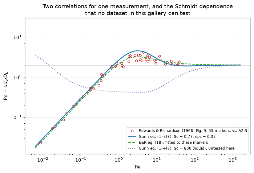
Gunn’s correlation sits +15.8% high on Edwards and Richardson’s points, 4.7 standard errors of the mean from zero, with a mean absolute deviation of 20.3%, against 11.75% for their own two-constant fit. That ordering is the expected one and is not a finding: E&R fitted \(\gamma\) and \(\beta\) to exactly these markers, while by Gunn’s own stated criterion, \(\mathrm{Re\,Sc}\gg1\), these points are unlikely to be in the set he estimated \(p(\mathrm{Re})\) from at all (47 of these 55 markers are below \(\mathrm{Re\,Sc} = 10\)).
What the comparison does establish is a ceiling, and a comparison it resolves only at a porosity of its own choosing.
The ceiling. Something Reynolds-dependent has to be in the model, or a constant must be chosen with care. Freezing \(p\) at 0.50, which is what the mixing-cell picture behind \(\mathrm{Pe} = 2\) amounts to, costs 68%, and E&R’s own uncorrected eq. (15) costs 30%. Both are far worse than 20%.
\(p(\mathrm{Re})\) against a constant. Over Re = 0.00857 to 49.1, \(p\) moves through 61% of its excursion, so these data do exercise \(p(\mathrm{Re})\). The right null is not \(p\) frozen at a printed plateau (24.9%); it is a free constant \(p\), which gives 22.96% at \(p\) = 0.0793. The mean absolute deviation of \(p(\mathrm{Re})\) is lower by 2.7 percentage points at \(\varepsilon\) = 0.37, which is 0.89 standard errors of the paired difference: these markers do not distinguish \(p(\mathrm{Re})\) from a constant. Given each the porosity it prefers (16.38% at \(\varepsilon\) = 0.443 against 21.01% at \(\varepsilon\) = 0.433) the difference is 4.6 points, 2.59 standard errors, so there the markers do prefer \(p(\mathrm{Re})\); which of the two comparisons applies is decided by a porosity the paper does not print.
And the unprinted porosity moves the headline more than either. The comparison gives 26.6% at \(\varepsilon\) = 0.34 and 17.5% at 0.40, a spread of 9.1 percentage points, larger than the 0.6 points that separate Gunn’s Schmidt group for argon–air from Edwards and Richardson’s, and larger than the ±5 px digitisation systematic (21.59% to 19.27%). The residual does not fall monotonically: it has an interior minimum at \(\varepsilon\) = 0.443 (16.4%), a looser bed than the 0.37 Gunn quotes for the bulk, and it rises again above that. With the porosity unprinted, nothing here can separate a porosity error from a model error, and the page does not try.
V5. The solver: two closed forms, and what each one cannot see
V5a: eq. (17), the paper’s own. With a flat inlet the 2-D bed has no radial gradient, so the radial operator annihilates the solution and the area-mean profile must be eq. (17) exactly. That is a real check on the axial discretisation and on the two axial boundary conditions, and it is structurally blind to everything radial: it cannot see nu=0, a wrong \(D_R\), or a five-cell radial grid.
V5b: a 2-D closed form, which can see them. Feed the bed the first zero-flux radial mode, \(c_0(r) = J_0(\beta_1 r/R)\) with \(J_1(\beta_1)=0\). The mode is an eigenfunction of the radial operator, so the exact solution is eq. (17) again with \(k \to k + D_R(\beta_1/R)^2\), a generalisation Gunn does not print, derived here, and one that reads \(D_R\), the geometry factor nu and the radial grid. Between them the two checks cover both axes; the break table measures which covers what instead of asserting it.
Each check reports two numbers: the largest error over all cells against the closed form at the cell centres (normalised by the largest value), and the outlet amplitude, the projection of the outlet face values on the feed profile (the area mean for a flat feed), whose exact value is \(U/(U+D\lambda)\,e^{-\lambda L}\). Orders come from successive differences of the outlet amplitude on a ladder of at least three grids (observed_orders), each axis of V5b on its own ladder and both together. The round-off companion is the gap between the two solver routes, Newton with the ConvFluxTVD Jacobian and van Leer deferred correction, on the same discrete equations.
@lru_cache(maxsize=None)
def solved(mode, n_z, n_r, route="newton"):
    """The bed at the operating point, flat (mode 0) or Bessel-mode (1) feed."""
    return bed(n_z=n_z, n_r=n_r, inlet_mode=mode).solve(route=route)


def amp_exact(b):
    return b.U / (b.U + b.D * b.lam) * np.exp(-b.lam * b.L)


def sup_err(b):
    ex = b.closed_form()
    return float(np.max(np.abs(b.c - ex)) / np.max(np.abs(ex)))


NZ_LAD = (100, 200, 400, 800)
ladders = {   # title: (feed mode, grids, the refined count that labels each grid)
    "V5a  flat feed, z refined (n_r = 20)": (0, [(n, 20) for n in NZ_LAD], 0),
    "V5b  Bessel mode, both refined": (1, [(n, n // 10) for n in NZ_LAD], 0),
    "V5b  Bessel mode, r refined (n_z = 800)": (1, [(800, n) for n in (10, 20, 40, 80)], 1),
    "V5b  Bessel mode, z refined (n_r = 80)": (1, [(n, 80) for n in NZ_LAD], 0),
}
LAD = {}
for title, (mode, grids, ax_) in ladders.items():
    vals = {g[ax_]: solved(mode, *g).outlet_amplitude() for g in grids}
    oo = observed_orders(lambda n: vals[n], [g[ax_] for g in grids])
    vals = list(vals.values())
    tab = pd.DataFrame({"n_z": [g[0] for g in grids], "n_r": [g[1] for g in grids],
                        "sup_error": [sup_err(solved(mode, *g)) for g in grids],
                        "outlet_rel_err": [v / amp_exact(solved(mode, *g)) - 1
                                           for v, g in zip(vals, grids)],
                        "newton_its": [solved(mode, *g).nit for g in grids]})
    LAD[title] = dict(tab=tab, orders=np.asarray(oo["orders"]),
                      finest_diff=abs(vals[-1] - vals[-2]))
    print(title)
    print(tab.drop(columns="newton_its").to_string(index=False, float_format=lambda v: f"{v:.4g}"))
    print(f"  observed orders of the outlet amplitude: "
          f"{', '.join(f'{o:.3f}' for o in LAD[title]['orders'])}\n")

EQ17_ERR = sup_err(solved(0, 800, 20))
BESSEL_ERR = sup_err(solved(1, 800, 80))
EQ17_OUT = abs(solved(0, 800, 20).outlet_amplitude() / amp_exact(solved(0, 800, 20)) - 1)
BESSEL_OUT = abs(solved(1, 800, 80).outlet_amplitude() / amp_exact(solved(1, 800, 80)) - 1)
GAP_ROUTES = max(float(np.max(np.abs(solved(m, *g).c - solved(m, *g, route="deferred").c)))
                 for m, g in ((0, (800, 20)), (1, (800, 80))))
NEWTON_ITS = max(int(LAD[t]["tab"].newton_its.max()) for t in LAD)
SWEEPS = max(solved(m, *g, route="deferred").nit for m, g in ((0, (800, 20)), (1, (800, 80))))
WALL_FINEST_DIFF = abs(wall_lad["values"][-1] - wall_lad["values"][-2])
FINEST_OVER_ROUNDOFF = min(min(LAD[t]["finest_diff"] for t in LAD),
                           WALL_FINEST_DIFF) / max(GAP_ROUTES, 1e-16)
print(f"Newton (ConvFluxTVD Jacobian) and deferred correction on the same discrete "
      f"equations, at (800, 20) and (800, 80): largest difference of a cell value "
      f"below 1e-12 (here {GAP_ROUTES:.1e})")
print(f"  Newton iterations at most 8 (here {NEWTON_ITS}); deferred-correction sweeps "
      f"to a change of 1e-12 (here {SWEEPS})")
print(f"  smallest last-step difference of any ladder, wall ladder included, over that gap: at least 1e3 "
      f"(here {FINEST_OVER_ROUNDOFF:.1e})")
V5a flat feed, z refined (n_r = 20)
n_z n_r sup_error outlet_rel_err
100 20 4.486e-05 -6.139e-05
200 20 1.163e-05 -1.546e-05
400 20 2.96e-06 -3.876e-06
800 20 7.454e-07 -9.701e-07
observed orders of the outlet amplitude: 1.987, 1.995
V5b Bessel mode, both refined
n_z n_r sup_error outlet_rel_err
100 10 0.001874 0.01298
200 20 0.0004657 0.003237
400 40 0.000116 0.0008086
800 80 2.896e-05 0.0002021
observed orders of the outlet amplitude: 2.005, 2.001
V5b Bessel mode, r refined (n_z = 800)
n_z n_r sup_error outlet_rel_err
800 10 0.001834 0.0132
800 20 0.0004595 0.00329
800 40 0.0001151 0.0008192
800 80 2.896e-05 0.0002021
observed orders of the outlet amplitude: 2.005, 2.001
V5b Bessel mode, z refined (n_r = 80)
n_z n_r sup_error outlet_rel_err
100 80 0.0001086 -1.762e-05
200 80 3.568e-05 0.0001494
400 80 2.982e-05 0.0001916
800 80 2.896e-05 0.0002021
observed orders of the outlet amplitude: 1.987, 1.995
Newton (ConvFluxTVD Jacobian) and deferred correction on the same discrete equations, at (800, 20) and (800, 80): largest difference of a cell value below 1e-12 (here 2.4e-14)
Newton iterations at most 8 (here 5); deferred-correction sweeps to a change of 1e-12 (here 9)
smallest last-step difference of any ladder, wall ladder included, over that gap: at least 1e3 (here 1.6e+07)The two routes agree to round-off and both converge here, so the choice between them is cost. Deferred correction reuses one LU of the upwind operator and needs about three times as many sweeps as Newton needs factorisations of the limited Jacobian; Newton with the exact Jacobian is the production route because its success flag is a convergence test of the limited equations themselves, and the swept fixed point is the independent second route.
V6. Break table for the solver checks
Every solver defect enters through a call argument of Bed. The rows marked “operator and closed form” change a coefficient consistently, in the operator, in \(\lambda\), in \(k_\mathrm{eff}\) and in closed_form(); the rows marked “operator only” build the operator with the wrong coefficient and keep the reference at the right one.
SOLVER_DEFECTS = [
    ("baseline", {}),
    ("nu = 0 on the radial divergence", dict(nu_r=0)),
    ("outlet eq. (18) -> zero gradient", dict(outlet="zero-gradient")),
    ("inlet Danckwerts -> Dirichlet", dict(inlet="dirichlet")),
    ("no TVD (bare first-order upwind)", dict(limiter=None)),
    ("radial grid n_r = 5", dict(n_r=5)),
    ("D_R +10 %, operator and closed form", dict(D_R=DR_OP * 1.1)),
    ("D +10 %, operator and closed form", dict(D=D_OP * 1.1)),
    ("D_R +10 % in the operator only", dict(DR_disc=DR_OP * 1.1)),
    ("D +10 % in the operator only", dict(D_disc=D_OP * 1.1)),
]


def solver_table(ref=((800, 20), (800, 80)), flat_kw=None):
    """sup errors of V5a and V5b under each defect, and the factors over baseline.

    ``flat_kw`` adds keywords to the flat-feed beds only (a break row).
    """
    rows = []
    for lab, kw in SOLVER_DEFECTS:
        kw = dict(kw)
        lim = kw.pop("limiter", "vanleer")
        e, o = [], []
        for mode, (nz, nr) in zip((0, 1), ref):
            kk = dict(n_z=nz, n_r=nr, inlet_mode=mode)
            kk.update(kw)
            if mode == 0 and flat_kw:
                kk.update(flat_kw)
            b = bed(**kk)
            b.solve() if lim == "vanleer" else b.solve(limiter=None)
            e.append(sup_err(b))
            o.append(abs(b.outlet_amplitude() / amp_exact(b) - 1))
        rows.append(dict(defect=lab, V5a=e[0], V5b=e[1], out_a=o[0], out_b=o[1]))
    sb = pd.DataFrame(rows)
    sb["x V5a"] = sb.V5a / sb.V5a[0]
    sb["x V5b"] = sb.V5b / sb.V5b[0]
    return sb


def solver_factors(sb):
    f = dict(zip(sb.defect, zip(sb["x V5a"], sb["x V5b"])))
    return {"bessel_break_nu0_factor": f["nu = 0 on the radial divergence"][1],
            "eq17_break_nu0_factor": f["nu = 0 on the radial divergence"][0],
            "bessel_break_zerograd_factor": f["outlet eq. (18) -> zero gradient"][1],
            "eq17_break_dirichlet_factor": f["inlet Danckwerts -> Dirichlet"][0],
            "bessel_break_upwind_factor": f["no TVD (bare first-order upwind)"][1],
            "bessel_break_n_r_5_factor": f["radial grid n_r = 5"][1],
            "bessel_consistent_DR_move": abs(f["D_R +10 %, operator and closed form"][1] - 1),
            "bessel_consistent_D_move": abs(f["D +10 %, operator and closed form"][1] - 1),
            "bessel_break_DR_operator_only_factor": f["D_R +10 % in the operator only"][1],
            "eq17_break_DR_operator_only_factor": f["D_R +10 % in the operator only"][0],
            "bessel_break_D_operator_only_factor": f["D +10 % in the operator only"][1],
            "eq17_break_D_operator_only_factor": f["D +10 % in the operator only"][0]}


SB = solver_table()
SF = solver_factors(SB)
print(SB.drop(columns=["out_a", "out_b"]).to_string(index=False,
                                                   float_format=lambda v: f"{v:.4g}"))

display(Markdown(rf"""
**Read the rows in pairs, because each check is blind where the other sees.** The
2-D check moves by factors of {SF['bessel_break_nu0_factor']:.0f},
{SF['bessel_break_zerograd_factor']:.0f}, {SF['bessel_break_upwind_factor']:.0f} and
{SF['bessel_break_n_r_5_factor']:.0f} for a wrong geometry factor, a wrong outlet
condition, bare upwind and a five-cell radial grid; eq. (17) moves by
{SF['eq17_break_dirichlet_factor']:.0f} for a Dirichlet inlet. `nu = 0` leaves
eq. (17)'s check at a factor of {SF['eq17_break_nu0_factor']:.6f}: a flat inlet
has no radial gradient, so the radial operator is multiplied by zero whatever
geometry it is given. A page carrying only that check could put `nu=0` in the
radial divergence and report a machine-precision agreement.

**The four coefficient rows are two different experiments and they say opposite
things.** Changed *consistently*, a 10 % error in $D_R$ or $D$ moves the 2-D
residual by {SF['bessel_consistent_DR_move']:.1%} and by below 0.1 %
(here {SF['bessel_consistent_D_move']:.4%}). That is the honest limit of these checks:
**a transport coefficient that is wrong *everywhere* is invisible to both**,
because the closed form they are compared against is built from the same numbers.
Nobody should read {BESSEL_ERR:.1e} as evidence that $D$ or $D_R$ is right.
Injected into the **operator alone**, the same 10 % moves eq. (17)'s check by a
factor {SF['eq17_break_D_operator_only_factor']:.0f} and the 2-D one by
{SF['bessel_break_D_operator_only_factor']:.1f} for $D$, and the 2-D one by
{SF['bessel_break_DR_operator_only_factor']:.0f} for $D_R$, while eq. (17)'s stays
at {SF['eq17_break_DR_operator_only_factor']:.6f}. A coefficient plumbed wrongly
*into* the operator is caught loudly; only a coefficient that is wrong in the
physics and in the reference alike gets through.
"""))
defect V5a V5b x V5a x V5b
baseline 7.454e-07 2.896e-05 1 1
nu = 0 on the radial divergence 7.454e-07 0.07662 1 2646
outlet eq. (18) -> zero gradient 0.00127 0.0006738 1704 23.27
inlet Danckwerts -> Dirichlet 0.01046 0.01618 1.403e+04 558.7
no TVD (bare first-order upwind) 0.001208 0.001843 1621 63.65
radial grid n_r = 5 7.454e-07 0.007284 1 251.5
D_R +10 %, operator and closed form 7.454e-07 3.079e-05 1 1.063
D +10 %, operator and closed form 7.425e-07 2.896e-05 0.9961 1
D_R +10 % in the operator only 7.454e-07 0.0129 1 445.3
D +10 % in the operator only 0.001021 0.001556 1369 53.74Read the rows in pairs, because each check is blind where the other sees. The 2-D check moves by factors of 2646, 23, 64 and 252 for a wrong geometry factor, a wrong outlet condition, bare upwind and a five-cell radial grid; eq. (17) moves by 14034 for a Dirichlet inlet. nu = 0 leaves eq. (17)’s check at a factor of 1.000000: a flat inlet has no radial gradient, so the radial operator is multiplied by zero whatever geometry it is given. A page carrying only that check could put nu=0 in the radial divergence and report a machine-precision agreement.
The four coefficient rows are two different experiments and they say opposite things. Changed consistently, a 10 % error in \(D_R\) or \(D\) moves the 2-D residual by 6.3% and by below 0.1 % (here 0.0058%). That is the honest limit of these checks: a transport coefficient that is wrong everywhere is invisible to both, because the closed form they are compared against is built from the same numbers. Nobody should read 2.9e-05 as evidence that \(D\) or \(D_R\) is right. Injected into the operator alone, the same 10 % moves eq. (17)’s check by a factor 1369 and the 2-D one by 53.7 for \(D\), and the 2-D one by 445 for \(D_R\), while eq. (17)’s stays at 1.000000. A coefficient plumbed wrongly into the operator is caught loudly; only a coefficient that is wrong in the physics and in the reference alike gets through.
V7. The outlet boundary condition, which is what eq. (18) is for
Gunn prints eq. (18) because Danckwerts’ \(\partial c/\partial x = 0\) is not the right downstream closure when dispersion is convection-dominated, and because the right one, \(c\to c_{eq}\) as \(x\to\infty\), cannot be imposed on a finite grid. Eq. (18) is the exact Robin condition the semi-infinite solution satisfies, so a bed of any length carrying it reproduces eq. (17). The paper says conditions (15) are “not easy to implement except where the reactor is long” and never says how long. The obvious reading, that a long bed makes the outlet condition stop mattering, turns out to be half right, and the half that is wrong is the half a reactor modeller cares about.
To first order in \(\lambda D/U\), imposing \(\partial c/\partial x = 0\) instead of \(\partial c/\partial x = -\lambda c\) mis-states the outlet gradient by exactly \(\lambda c\), and the resulting error at the outlet is a multiplicative bias of order \(\lambda D/U\), a group containing the rate constant and the dispersion coefficient and not the bed length. The tables below sweep both, on 32 cells per particle diameter. With a flat feed and a uniform velocity the bed has no radial gradient, so one radial cell carries the same solution as twenty; the cell below measures that before relying on it. The interior probe is the value at \(z = 4\) particle diameters, a cell face on these grids, read as the mean of the two cells beside it.
CELLS_PER_D = 32
PROBE_Z = 4.0


def outlet_pair(L, k, per_d=CELLS_PER_D, n_r=1, lam_scale=1.0, probe_z=PROBE_Z, at="face",
                **kw):
    """The same bed with eq. (18) and with a zero-gradient outlet; outlet values on the face.

    ``lam_scale``, ``at`` and ``kw`` (passed to ``Bed``) exist for the break table.
    """
    n_z = int(per_d * L)
    bg = bed(L=L, k=k, n_z=n_z, n_r=n_r, outlet="gunn", lam_scale=lam_scale, **kw).solve()
    bd = bed(L=L, k=k, n_z=n_z, n_r=n_r, outlet="zero-gradient", **kw).solve()
    cg, cd = bg.outlet_amplitude(at), bd.outlet_amplitude(at)
    i = int(round(probe_z * per_d))           # z = probe_z is face i
    pg, pd_ = 0.5 * (bg.c[i - 1, 0] + bg.c[i, 0]), 0.5 * (bd.c[i - 1, 0] + bd.c[i, 0])
    return dict(gunn_vs_eq17=abs(cg / amp_exact(bg) - 1), outlet_error=cd / cg - 1,
                lam_D_over_U=bg.lam * bg.D / bg.U, error_at_probe=pd_ / pg - 1)


ONE_VS_TWENTY = abs(outlet_pair(L_OP, K_OP, n_r=20)["outlet_error"]
                    / outlet_pair(L_OP, K_OP)["outlet_error"] - 1)
print(f"one radial cell against twenty, flat feed: outlet error differs by below 1e-10 "
      f"relative (here {ONE_VS_TWENTY:.1e})\n")

print("(a) bed length swept, everything else fixed - k L/U therefore varies")
LODS = (5.0, 10.0, 20.0, 50.0, 100.0, 200.0)
ta = pd.DataFrame([dict(L_over_d=Lod, **outlet_pair(Lod, K_OP)) for Lod in LODS])
print(ta.drop(columns="error_at_probe").to_string(index=False, float_format=lambda v: f"{v:.4g}"))
print("  error at the probe z = 4:")
for Lod, v in zip(ta.L_over_d, ta.error_at_probe):
    if Lod <= 10:
        print(f"    L/d = {Lod:5.0f}   {v:+.4g}")
    else:
        print(f"    L/d = {Lod:5.0f}   below 1e-14 in magnitude (here {v:.1e})")

print("\n(b) reaction rate swept at a fixed 100-diameter bed")
DAS = (0.05, 0.2, 1.0, 2.0, 5.0, 20.0)
tb = pd.DataFrame([dict(k_L_over_U=Da, **outlet_pair(L_OP, Da / L_OP)) for Da in DAS])
tb["error_over_lam_D_U"] = tb.outlet_error / tb.lam_D_over_U
print(tb.drop(columns="error_at_probe").to_string(index=False, float_format=lambda v: f"{v:.4g}"))

BC_ERR_SHORT, BC_ERR_LONG = float(ta.outlet_error.iloc[0]), float(ta.outlet_error.iloc[-1])
BC_LEN_SPREAD = float(np.max(np.abs(ta.outlet_error / ta.outlet_error.iloc[-1] - 1)))
BC_PROBE_SHORT, BC_PROBE_MID = float(ta.error_at_probe.iloc[0]), float(ta.error_at_probe.iloc[1])
BC_PROBE_LONG = float(np.max(np.abs(ta.error_at_probe.iloc[2:])))
BC_RATIO_LO, BC_RATIO_HI = float(tb.error_over_lam_D_U.min()), float(tb.error_over_lam_D_U.max())
EQ18_VS_EQ17 = float(ta.gunn_vs_eq17.max())
display(Markdown(rf"""
**At the outlet the mistake does not shrink with bed length at all.** Table (a)
holds $k$, $D$ and $U$ fixed and grows the bed from {LODS[0]:.0f} to {LODS[-1]:.0f}
particle diameters: the zero-gradient outlet reports {BC_ERR_SHORT:+.2%} too much
unreacted material at the short end and {BC_ERR_LONG:+.2%} at the long end, the
same to below 1e-5 relative across the table (here {BC_LEN_SPREAD:.0e}). A
{LODS[-1] / LODS[0]:.0f}-fold longer bed buys nothing, because the error is a
multiplicative bias set by the mismatch in the imposed gradient, not an entrance
effect that has time to decay.

**What the length does buy is the interior.** At a fixed station 4 diameters from
the inlet the same error is {BC_PROBE_SHORT:+.2%} when that station is one diameter
from the end of a {LODS[0]:.0f}-diameter bed, {BC_PROBE_MID:.1e} in a
{LODS[1]:.0f}-diameter bed, and at round-off from {LODS[2]:.0f} diameters on. **That**
is what "except where the reactor is long" means: the perturbation is confined to
a few dispersion lengths at the end, so a long bed protects the profile you are
looking at and never the outlet itself.

**And the size of it is $\lambda D/U$, with no fitted constant.** Table (b) sweeps
$kL/U$ over {DAS[0]:g} to {DAS[-1]:g} at one bed length, a
{DAS[-1] / DAS[0]:.0f}-fold range: the outlet error runs from
{float(tb.outlet_error.iloc[0]):+.3%} to {float(tb.outlet_error.iloc[-1]):+.2%}, and
the ratio of the measured error to $\lambda D/U$ stays between {BC_RATIO_LO:.3f} and
{BC_RATIO_HI:.3f} throughout. So the group predicts the scaling and bounds the
magnitude to within {1 - BC_RATIO_LO:.0%}: a modeller who wants to know whether the
outlet condition matters should compute it rather than count particle diameters.

The zero-gradient condition is a **different physical problem**, not a worse
approximation to the same one, and `A2.1` is the page about what that difference
means. Meanwhile eq. (18) reproduces eq. (17) at the outlet to
{EQ18_VS_EQ17:.1e} at every length in table (a), which is what makes it usable on
a short grid.
"""))
one radial cell against twenty, flat feed: outlet error differs by below 1e-10 relative (here 4.1e-13)
(a) bed length swept, everything else fixed - k L/U therefore varies
L_over_d gunn_vs_eq17 outlet_error lam_D_over_U
5 2.567e-09 0.01035 0.01046
10 5.625e-09 0.01035 0.01046
20 1.174e-08 0.01035 0.01046
50 3.009e-08 0.01035 0.01046
100 6.066e-08 0.01035 0.01046
200 1.218e-07 0.01035 0.01046
error at the probe z = 4:
L/d = 5 +0.001502
L/d = 10 +9.653e-08
L/d = 20 below 1e-14 in magnitude (here -2.2e-16)
L/d = 50 below 1e-14 in magnitude (here 0.0e+00)
L/d = 100 below 1e-14 in magnitude (here 0.0e+00)
L/d = 200 below 1e-14 in magnitude (here 0.0e+00)
(b) reaction rate swept at a fixed 100-diameter bed
k_L_over_U gunn_vs_eq17 outlet_error lam_D_over_U error_over_lam_D_U
0.05 4.399e-12 0.0002641 0.0002642 0.9997
0.2 5.3e-11 0.001055 0.001056 0.9989
1 7.815e-09 0.00523 0.005258 0.9948
2 6.066e-08 0.01035 0.01046 0.9896
5 8.663e-07 0.02512 0.02576 0.9749
20 3.714e-05 0.08793 0.09641 0.912At the outlet the mistake does not shrink with bed length at all. Table (a) holds \(k\), \(D\) and \(U\) fixed and grows the bed from 5 to 200 particle diameters: the zero-gradient outlet reports +1.04% too much unreacted material at the short end and +1.04% at the long end, the same to below 1e-5 relative across the table (here 7e-07). A 40-fold longer bed buys nothing, because the error is a multiplicative bias set by the mismatch in the imposed gradient, not an entrance effect that has time to decay.
What the length does buy is the interior. At a fixed station 4 diameters from the inlet the same error is +0.15% when that station is one diameter from the end of a 5-diameter bed, 9.7e-08 in a 10-diameter bed, and at round-off from 20 diameters on. That is what “except where the reactor is long” means: the perturbation is confined to a few dispersion lengths at the end, so a long bed protects the profile you are looking at and never the outlet itself.
And the size of it is \(\lambda D/U\), with no fitted constant. Table (b) sweeps \(kL/U\) over 0.05 to 20 at one bed length, a 400-fold range: the outlet error runs from +0.026% to +8.79%, and the ratio of the measured error to \(\lambda D/U\) stays between 0.912 and 1.000 throughout. So the group predicts the scaling and bounds the magnitude to within 9%: a modeller who wants to know whether the outlet condition matters should compute it rather than count particle diameters.
The zero-gradient condition is a different physical problem, not a worse approximation to the same one, and A2.1 is the page about what that difference means. Meanwhile eq. (18) reproduces eq. (17) at the outlet to 1.2e-07 at every length in table (a), which is what makes it usable on a short grid.
V8. A second, independent route
Every row of a break table perturbs an input and watches a number move. No row of that kind can tell you that the baseline is wrong. A defect-injection table answers “is this check sensitive?”; it never answers “is this number right?”. The thing that answers the second question is computing the quantity a second time by a route that shares no code with the first.
So two reactor numbers are recomputed with scipy.integrate.solve_bvp: collocation on a different mesh, in a different solver, with a different error mechanism, reproducing the pymrm bed’s own boundary statements exactly so that the comparison isolates the discretisation. The reference raises unless status == 0 and its rms residuals are printed.
The first is the outlet-condition error of V7. It also shows why the outlet value is read on the face: the last cell centre sits \(h/2\) short of \(z = L\), and since eq. (18) and the zero-gradient outlet differ in their outlet gradient by construction, that offset does not cancel in their ratio. The table reads the same pairs of solves both ways on four grids.
The second is the wall-channel cost with radial dispersion off. With \(D_R\to0\) the columns decouple, so each velocity gets its own one-dimensional collocation solve and the outlet is flux-weighted by hand. That route reads the velocity profile, the area weights and cup(), none of which V5a or V5b touch, because both of them run a uniform profile.
def bvp_outlet(u_local, D, k, L, U, lam, outlet, n0=400, tol=1e-10):
    """D c'' - u c' - k c = 0 by collocation. Returns (c(L), worst rms residual).

    Shares no assembly, no operator and no solver with `Bed`. The inlet balance
    is written with the area-mean U exactly as `Bed` writes it. Raises if the
    reference solver did not reach its own tolerance.
    """
    def rhs(z, y):
        return np.vstack([y[1], (u_local * y[1] + k * y[0]) / D])

    def bcf(ya, yb):
        left = U * ya[0] - D * ya[1] - U                                 # Danckwerts, c0 = 1
        right = yb[1] + lam * yb[0] if outlet == "gunn" else yb[1]   # eq. (18) or dc/dz = 0
        return np.array([left, right])

    z = np.linspace(0.0, L, n0)
    y = np.vstack([np.exp(-lam * z), -lam * np.exp(-lam * z)])
    s = solve_bvp(rhs, bcf, z, y, tol=tol, max_nodes=400_000)
    if s.status != 0:
        raise RuntimeError(f"collocation reference did not converge: {s.message}")
    return float(s.sol(L)[0]), float(np.max(s.rms_residuals))


def collocation_outlet_error():
    lam = bed(n_z=4, n_r=1).lam
    cg, rg = bvp_outlet(1.0, D_OP, K_OP, L_OP, 1.0, lam, "gunn")
    cd, rd = bvp_outlet(1.0, D_OP, K_OP, L_OP, 1.0, lam, "zero-gradient")
    return cd / cg - 1.0, max(rg, rd)


BC_ERR_BVP, RMS_BVP = collocation_outlet_error()
ref = []
for per_d in (8, 16, 32, 64):
    n_z = int(per_d * L_OP)
    bg = bed(n_z=n_z, n_r=1, outlet="gunn").solve()
    bd = bed(n_z=n_z, n_r=1, outlet="zero-gradient").solve()
    ref.append(dict(cells_per_d=per_d, at_cell_centre=float(bd.c[-1, 0] / bg.c[-1, 0] - 1),
                    on_face=float(bd.outlet_amplitude() / bg.outlet_amplitude() - 1)))
ref = pd.DataFrame(ref)
ref["centre_vs_bvp"] = dev(ref.at_cell_centre, BC_ERR_BVP)
ref["face_vs_bvp"] = dev(ref.on_face, BC_ERR_BVP)
print(f"collocation reference (independent): outlet error = {BC_ERR_BVP:.8f}"
      f"   (status 0, worst rms residual below 1e-9, here {RMS_BVP:.1e})")
print(ref.to_string(index=False, float_format=lambda v: f"{v:.6g}"))
BC_FV_VS_BVP = float(ref.face_vs_bvp[ref.cells_per_d == CELLS_PER_D].iloc[0])
BC_CENTRE_VS_BVP_H8 = float(ref.centre_vs_bvp.iloc[0])
BC_CENTRE_VS_BVP = float(ref.centre_vs_bvp[ref.cells_per_d == CELLS_PER_D].iloc[0])


def bvp_cup(ratio_w, extent=None):
    """Flux-weighted outlet of the wall bed with decoupled columns, by collocation."""
    b = bed(n_z=4, n_r=WALL_GRID[1], wall_ratio=ratio_w,
            wall_extent=G["wall_region_extent_diameters"] if extent is None else extent)
    cache, worst = {}, 0.0
    for u in np.unique(b.U * b.prof):
        cache[u], rms = bvp_outlet(u, b.D, b.k, b.L, b.U, b.lam, "gunn")
        worst = max(worst, rms)
    cL = np.array([cache[u] for u in b.U * b.prof])
    flux = b.w * b.prof
    return float((cL * flux).sum() / flux.sum()), worst, len(cache)


cup_w, rms_w, n_vel = bvp_cup(R165)
cup_u, rms_u, _ = bvp_cup(1.0)
WALL_NO_RADIAL_BVP = cup_w / cup_u - 1.0
WALL_FV_VS_BVP = float(dev(NAIVE_WITHOUT, WALL_NO_RADIAL_BVP))
RMS_BVP = max(RMS_BVP, rms_w, rms_u)
print(f"\nwall channel, radial dispersion off, {n_vel} distinct column velocities solved "
      "separately by collocation")
print(f"  pymrm 2-D bed  {NAIVE_WITHOUT:+.8f}")
print(f"  collocation    {WALL_NO_RADIAL_BVP:+.8f}")
print(f"  they differ by {abs(WALL_FV_VS_BVP):.2e} relative")

display(Markdown(rf"""
**The independent route agrees on both numbers, and shows what the face read is
worth.**

The wall-channel cost with radial dispersion off is {NAIVE_WITHOUT:+.4%} from the
2-D finite-volume bed and {WALL_NO_RADIAL_BVP:+.4%} from independent per-column
collocation, **{abs(WALL_FV_VS_BVP):.1e} relative**. That is the check on this page
that reads the velocity profile, the area weights and the mixing-cup weighting;
V5a and V5b cannot, because both are run with a uniform profile, and no break row
would have revealed it either, since a break row only asks whether a number
*moves*.

The outlet-condition error is {BC_ERR_BVP:.4%} by collocation. Read on the outlet
**face** with `compute_boundary_values`, the finite-volume pair gives
{BC_FV_VS_BVP:+.1e} of that at $h = 1/{CELLS_PER_D}$ particle diameters, falling
with $h$ in the table. The same solves read at the last cell **centre** land
{BC_CENTRE_VS_BVP:+.1%} away at the same grid and {BC_CENTRE_VS_BVP_H8:+.1%} away
at $h = 1/{ref.cells_per_d.iloc[0]:.0f}$: a first-order bias of order
$\lambda h/2$ that survives every sweep V7 performs, because V7 holds $h$ fixed
while it varies $L$ and $k$.

*The general lesson.* A defect-injection table measures **sensitivity**; it is
silent about **accuracy**. A metric can move loudly for every wrong input and still
be wrong for every right one. Perturbation testing cannot see a quantity read at
the wrong location, a convergence floor mistaken for an answer, or a reference and
an operator that share a mistake. A second, independent computation can.
"""))
collocation reference (independent): outlet error = 0.01035288 (status 0, worst rms residual below 1e-9, here 9.9e-11)
cells_per_d at_cell_centre on_face centre_vs_bvp face_vs_bvp
8 0.0091704 0.0103526 -0.114218 -2.82764e-05
16 0.0097457 0.0103528 -0.058649 -1.12126e-05
32 0.010045 0.0103528 -0.0297418 -3.48365e-06
64 0.0101978 0.0103529 -0.0149794 -9.77694e-07
wall channel, radial dispersion off, 2 distinct column velocities solved separately by collocation
pymrm 2-D bed +0.05461435
collocation +0.05461427
they differ by 1.54e-06 relativeThe independent route agrees on both numbers, and shows what the face read is worth.
The wall-channel cost with radial dispersion off is +5.4614% from the 2-D finite-volume bed and +5.4614% from independent per-column collocation, 1.5e-06 relative. That is the check on this page that reads the velocity profile, the area weights and the mixing-cup weighting; V5a and V5b cannot, because both are run with a uniform profile, and no break row would have revealed it either, since a break row only asks whether a number moves.
The outlet-condition error is 1.0353% by collocation. Read on the outlet face with compute_boundary_values, the finite-volume pair gives -3.5e-06 of that at \(h = 1/32\) particle diameters, falling with \(h\) in the table. The same solves read at the last cell centre land -3.0% away at the same grid and -11.4% away at \(h = 1/8\): a first-order bias of order \(\lambda h/2\) that survives every sweep V7 performs, because V7 holds \(h\) fixed while it varies \(L\) and \(k\).
The general lesson. A defect-injection table measures sensitivity; it is silent about accuracy. A metric can move loudly for every wrong input and still be wrong for every right one. Perturbation testing cannot see a quantity read at the wrong location, a convergence floor mistaken for an answer, or a reference and an operator that share a mistake. A second, independent computation can.
Claims: what each number is, and how it is checked
Every number the page states is registered once here (docs/claims-design.md): a value (physics, data, arithmetic on printed numbers or a discretisation result, held by CI to a relative tolerance), a bound (a residual, a two-route gap, a round-off effect or a convergence order, checked at run time) or an exact result (a count or a verdict, with its distance to the threshold that decides it). Arithmetic on printed constants and the data comparison are held to 1e-4 relative, solver results to 1e-3, two-route gaps and the grid-error estimates to 5 %.
FIXED, SOLV, LOOSE = 1e-4, 1e-3, 0.05


def phrase_check(cs, t1, G):
    """Half-units of the last printed digit, and the deviations, of the stated numbers."""
    p_inf = G["p_offset"] + G["p_amplitude_spheres"]
    rows = [(cs["pe_at_Re_1000"], G["peclet_high_re_asymptote"], 1.0),
            (float(p_of_Re(G["reynolds_p_lower_plateau"], G)), G["p_offset"], 0.01),
            (float(p_of_Re(G["reynolds_p_upper_plateau"], G)), p_inf, 0.01),
            (cs["liquid_gas_max_ratio"], G["liquid_gas_max_factor"], 1.0),
            (cs["liquid_gas_max_reynolds"], G["liquid_gas_max_reynolds"], 1.0),
            (cs["liquid_gas_crossover_reynolds"], G["liquid_gas_range_min"], 0.1),
            (t1["table1_mean"], G["intraparticle_diffusivity_fraction"], 0.01)]
    comp, printed, unit = (np.array(c, float) for c in zip(*rows))
    return np.abs(comp - printed) / (unit / 2), np.abs(comp / printed - 1)


def op_point(G, eps=EPS, eq1=None):
    eq1 = dict(eq1 or {})
    return {"pe_axial_operating_point": float(Pe_axial(RE_OP, G["schmidt_argon_air"], G, eps, **eq1)),
            "pe_radial_operating_point": float(Pe_radial(RE_OP, G["schmidt_argon_air"], G, eps))}


def value(name, x, rtol=FIXED, **kw):
    claims.value(name, x, rtol=rtol, **kw)


def bound(name, x, **kw):
    claims.bound(name, x, **kw)


# --- the correlations, from printed constants only -------------------------------
for k in ("pe_limit_spheres", "pe_limit_solid_cylinders", "pe_limit_hollow_cylinders",
          "pe_limit_spread_spheres_over_hollow", "pe_limit_rounding_width",
          "D_axial_over_D_radial_high_Re", "pe_at_Re_1000", "p_at_Re_1000_rel_dev",
          "fraction_of_p_excursion_1_to_200", "liquid_gas_max_ratio",
          "liquid_gas_max_reynolds", "liquid_gas_crossover_reynolds",
          "liquid_gas_ratio_at_Re_300", "liquid_gas_ratio_at_Re_1000", "eq1_peclet_maximum",
          "eq1_peclet_maximum_reynolds", "eq1_peclet_minimum", "eq1_peclet_minimum_reynolds",
          "reynolds_pe_within_5e-4_of_2", "wall_velocity_ratio_rel_dev",
          "tau_inverse_vs_er_gamma_rel_dev", "low_re_slope_gunn_over_er"):
    value(k, CS[k])
value("p_at_Re_1_rel_dev", CS["p_at_Re_1_rel_dev"], rtol=0.01,
      note="(0.33/0.17) exp(-24): the plateau below Re = 1")
bound("pe_limit_vs_eq1_worst_rel_dev", CS["pe_limit_vs_eq1_worst_rel_dev"], max=1e-7,
      basis="theory", note="eq. (1) at Re = 1e8 approaches its limit as 1/Re")
for k in ("pe_limit_spheres_over_solid_worst_rounding", "pe_limit_solid_over_hollow_worst_rounding"):
    bound(k, CS[k], min=1.0, basis="theory",
          note="the order of two shapes' limits survives the rounding of both")
bound("eq1_vs_eq42_identity", CS["eq1_vs_eq42_identity"], max=1e-9, basis="identity",
      note="algebraically identical forms; the gap is round-off in their cancellation")
bound("expm1_vs_naive_exp_worst", CS["expm1_vs_naive_exp_worst"], min=1e-7, max=1e-4,
      basis="theory", note="exp(x) - 1 at |x| near 1e-10 loses about 1e-16/|x|")
claims.exact("liquid_gas_crossings", CS["liquid_gas_crossings"],
             note="sign changes of the liquid/gas ratio minus one on Re = 1e-3 to 1e6")
HU, PDEV = phrase_check(CS, T1, G)
claims.count("stated_numbers_within_half_unit", HU, 1.0, above=False, min_margin=0.1,
             note="half-units of the last printed digit; margin to 1 half-unit")
value("stated_numbers_worst_rel_dev", PDEV.max())
for k, v in op_point(G).items():
    value(k, v)
# --- Table 1 ------------------------------------------------------------------
for k in ("table1_worst_row_spread", "table1_mean_row_spread", "table1_mean_vs_stated_rel_dev"):
    value(k, T1[k])
claims.exact("table1_rows_counterdiffusion_largest", T1["table1_rows_counterdiffusion_largest"])
# --- against measurement --------------------------------------------------------
for k in ("eq1_vs_fig9_mean_abs_dev", "eq1_vs_fig9_bias", "eq1_vs_fig9_bias_over_se",
          "eq18_vs_fig9_mean_abs_dev_recomputed", "null_p_frozen_low_mean_abs_dev",
          "null_p_frozen_high_mean_abs_dev", "null_eq15_mean_abs_dev",
          "null_free_constant_p_value", "null_free_constant_p_mean_abs_dev",
          "null_free_constant_p_sensitivity", "p_cost_vs_free_constant",
          "p_cost_vs_free_constant_over_se", "eq1_vs_fig9_mad_eps_034",
          "eq1_vs_fig9_mad_eps_040", "eq1_vs_fig9_best_eps", "eq1_vs_fig9_mad_at_best_eps",
          "null_free_constant_p_best_eps", "null_free_constant_p_best_p",
          "null_free_constant_p_best_eps_mean_abs_dev", "p_cost_at_preferred_eps",
          "p_cost_at_preferred_eps_over_se", "fraction_of_p_excursion_sampled",
          "eq1_vs_fig9_mad_shift_minus5px", "eq1_vs_fig9_mad_shift_plus5px",
          "eq1_vs_fig9_mad_fused_included", "resc_min", "resc_max", "resc_median"):
    value(k, DS[k])
claims.exact("n_fig9_markers_used", len(Pe_d))
claims.count("n_resc_below_1", Re_d * SC, 1.0, above=False, min_margin=0.01)
claims.count("n_resc_below_10", Re_d * SC, 10.0, above=False, min_margin=0.01)
claims.exact("null_free_constant_p_local_minima", DS["null_free_constant_p_local_minima"],
             note="local minima of the mean absolute deviation on the scan of p")
claims.exact("eq1_vs_fig9_eps_local_minima", DS["eq1_vs_fig9_eps_local_minima"],
             note="local minima of the mean absolute deviation on the scan of eps")
SE2 = 2.0      # a difference is called resolved beyond two standard errors
claims.exact("bias_resolved", bool(DS["eq1_vs_fig9_bias_over_se"] > SE2),
             margin=abs(DS["eq1_vs_fig9_bias_over_se"] - SE2), min_margin=0.2,
             note="mean bias beyond two standard errors of the mean")
claims.exact("p_cost_resolved_at_assumed_eps", bool(DS["p_cost_vs_free_constant_over_se"] > SE2),
             margin=abs(DS["p_cost_vs_free_constant_over_se"] - SE2), min_margin=0.2,
             note="p(Re) against a free constant p, two standard errors of the paired difference")
claims.exact("p_cost_resolved_at_preferred_eps",
             bool(DS["p_cost_at_preferred_eps_over_se"] > SE2),
             margin=abs(DS["p_cost_at_preferred_eps_over_se"] - SE2), min_margin=0.2,
             note="the same, each model at the porosity it prefers")
bound("eq18_recompute_vs_A25_gap", GAP25, max=1e-12, basis="identity",
      note="the same arithmetic on the same file as A2.5's committed claims")
bound("eq18_peak_vs_A25_gap", GAP25_PEAK, max=1e-8, basis="tolerance",
      note="closed-form maximum against A2.5's committed root")
bound("derivative_vs_mpmath", DERIV_CHECK, max=1e-7, basis="tolerance",
      note="analytic d(D/Ud)/dRe against mpmath, scaled by D/(Ud)/Re")
bound("eq17_identities_worst", EQ17_ID, max=1e-10, basis="identity",
      note="eq. (17) in eq. (16) and in the Danckwerts inlet, algebraically")
# --- the solver -------------------------------------------------------------------
value("eq17_flat_sup_error", EQ17_ERR, rtol=SOLV)
value("bessel_mode_sup_error", BESSEL_ERR, rtol=SOLV)
value("eq17_flat_outlet_rel_err", EQ17_OUT, rtol=SOLV)
value("bessel_outlet_rel_err", BESSEL_OUT, rtol=SOLV)
V5_ORDERS = np.concatenate([LAD[t]["orders"] for t in LAD])
bound("v5_order_min", V5_ORDERS.min(), min=1.9, basis="theory",
      note="second order; successive differences of the outlet amplitude, four ladders")
bound("v5_order_max", V5_ORDERS.max(), max=2.1, basis="theory",
      note="second order; successive differences of the outlet amplitude, four ladders")
bound("newton_vs_deferred_gap", GAP_ROUTES, max=1e-12, basis="tolerance",
      note="two solvers of the same limited equations, step tolerance 1e-12")
bound("ladder_finest_over_roundoff", FINEST_OVER_ROUNDOFF, min=1e3, basis="theory",
      note="last-step difference of every ladder over the two-route gap")
bound("newton_iterations_worst", NEWTON_ITS, max=8, basis="chosen",
      note="Newton from the upwind solution with the exact ConvFluxTVD Jacobian")
for k, v in SF.items():
    if k in ("eq17_break_nu0_factor", "eq17_break_DR_operator_only_factor"):
        bound(k, v, min=1 - 1e-6, max=1 + 1e-6, basis="identity",
              note="a flat feed has no radial gradient, so the radial operator is idle")
    elif k == "bessel_consistent_D_move":
        bound(k, v, max=1e-3, basis="theory",
              note="a D wrong in operator and closed form alike barely moves the 2-D check")
    else:
        value(k, v, rtol=SOLV)
# --- the wall channel ---------------------------------------------------------------
value("wall_channel_cost_with_radial", NAIVE_WITH, rtol=SOLV)
value("wall_channel_cost_without_radial", NAIVE_WITHOUT, rtol=SOLV)
value("wall_cost_gunn_ratio_with_radial", GUNN_WITH, rtol=SOLV)
value("wall_cost_gunn_ratio_without_radial", GUNN_WITHOUT, rtol=SOLV)
value("radial_erosion_fraction", HEAL, rtol=SOLV)
value("wall_cost_local_inlet_with_radial", NAIVE_WITH_LOCAL, rtol=SOLV)
value("wall_cost_local_inlet_without_radial", NAIVE_WITHOUT_LOCAL, rtol=SOLV)
value("local_inlet_effect", LOCAL_MOVE, rtol=SOLV)
value("wall_cost_n_r_40", wall_lad["values"][1], rtol=SOLV)
value("wall_cost_richardson_estimate", WALL_EXTRAP, rtol=SOLV)
value("wall_cost_grid_error", WALL_GRID_ERR, rtol=LOOSE)
bound("wall_cost_r_order_min", WALL_R_ORDERS.min(), min=1.8, basis="theory",
      note="second order in the radial grid, the annulus edge on a cell face")
bound("wall_cost_r_order_max", WALL_R_ORDERS.max(), max=2.2, basis="theory",
      note="second order in the radial grid, the annulus edge on a cell face")
# --- the outlet condition -------------------------------------------------------------
value("zerograd_outlet_error_short_bed", BC_ERR_SHORT, rtol=SOLV)
value("zerograd_outlet_error_long_bed", BC_ERR_LONG, rtol=SOLV)
bound("zerograd_outlet_error_length_spread", BC_LEN_SPREAD, max=1e-5, basis="chosen",
      note="the length dependence the page calls none, over L/d = 5 to 200")
value("zerograd_error_at_probe_5d_bed", BC_PROBE_SHORT, rtol=SOLV)
value("zerograd_error_interior_10d_bed", BC_PROBE_MID, rtol=SOLV)
bound("zerograd_error_interior_long_beds", BC_PROBE_LONG, max=1e-14, basis="theory",
      note="the outlet perturbation decays over a few dispersion lengths; round-off")
value("zerograd_error_over_lambda_D_U_min", BC_RATIO_LO, rtol=SOLV)
value("zerograd_error_over_lambda_D_U_max", BC_RATIO_HI, rtol=SOLV)
value("eq18_vs_eq17_outlet_worst", EQ18_VS_EQ17, rtol=SOLV)
bound("one_vs_twenty_radial_cells", ONE_VS_TWENTY, max=1e-10, basis="identity",
      note="flat feed and uniform velocity: no radial gradient")
# --- the independent route ---------------------------------------------------------------
value("outlet_error_collocation", BC_ERR_BVP)
value("outlet_error_fv_vs_collocation", BC_FV_VS_BVP, rtol=LOOSE)
value("outlet_error_centre_vs_collocation_h8", BC_CENTRE_VS_BVP_H8, rtol=SOLV)
value("outlet_error_centre_vs_collocation_h32", BC_CENTRE_VS_BVP, rtol=SOLV)
value("wall_cost_no_radial_collocation", WALL_NO_RADIAL_BVP)
value("wall_cost_fv_vs_collocation", WALL_FV_VS_BVP, rtol=LOOSE)
bound("collocation_rms_worst", RMS_BVP, max=1e-9, basis="tolerance",
      note="solve_bvp tol 1e-10")
print(f"{len(claims.metrics)} claims registered")
128 claims registeredThe defect-injection table
Every claim above needs a row that fails its own check. Two families of claim live on this page and they fail under disjoint defects. The correlation and data claims come from three studies (correlation_study, data_study and table1_study) that take the printed constants as a dictionary: each row below mis-reads one constant, or changes one argument of eq. (1), and reruns every study in full. A study that cannot be computed under a defect (a crossing that disappears, a minimum that moves to the edge of its window) records nan, which fails its claim, and the refusal is listed. The solver and reactor claims get rows of their own, each a call argument of Bed, of the outlet pair or of the collocation route.
BREAK = []


def brk(row, name, broken):
    """One injected defect: ``broken`` is what claim ``name`` becomes with it."""
    if isinstance(broken, (float, np.floating)) and not np.isfinite(broken):
        broken = np.nan
    caught = claims.breaks(row, name, broken)
    BREAK.append((row, name, caught))


def study_row(label, G=G, eps=EPS, eq1=None, alpha1_1993=None, E=E, re=Re_d, pe=Pe_d,
              t1=tab1, px=None):
    """Rerun every closed-form and data study under one defect; register each claim."""
    cs = correlation_study(G, eps=eps, eq1=eq1, alpha1_1993=alpha1_1993, E=E)
    ds = data_study(G, eps=eps, eq1=eq1, E=E, re=re, pe=pe, px_per_decade=px)
    t1s = table1_study(t1, G)
    refused = cs["_refused"] + ds["_refused"]
    res = {**cs, **ds, **t1s, **op_point(G, eps, eq1)}
    hu, pdev = phrase_check(cs, t1s, G) if not refused else (np.full(7, np.nan),) * 2
    res["stated_numbers_within_half_unit"] = (int(np.sum(hu <= 1.0)) if np.all(np.isfinite(hu))
                                              else np.nan)
    res["stated_numbers_worst_rel_dev"] = float(np.max(pdev))
    res["n_fig9_markers_used"] = len(pe)
    res["n_resc_below_1"], res["n_resc_below_10"] = ds["n_resc_below_1"], ds["n_resc_below_10"]
    for k, x in (("bias_resolved", ds["eq1_vs_fig9_bias_over_se"]),
                 ("p_cost_resolved_at_assumed_eps", ds["p_cost_vs_free_constant_over_se"]),
                 ("p_cost_resolved_at_preferred_eps", ds["p_cost_at_preferred_eps_over_se"])):
        res[k] = bool(x > SE2) if np.isfinite(x) else np.nan
    res["eq18_recompute_vs_A25_gap"] = max(
        abs(ds["eq18_vs_fig9_mean_abs_dev_recomputed"] - C25["eq18_vs_fig9_mean_abs_dev"]),
        abs(ds["eq18_vs_fig9_bias_recomputed"] - C25["eq18_vs_fig9_bias"]))
    res["eq18_peak_vs_A25_gap"] = max(
        abs(ds["eq18_pe_max_recomputed"] / C25["eq18_pe_max"] - 1),
        abs(ds["eq18_re_at_pe_max_recomputed"] / C25["eq18_re_at_pe_max"] - 1))
    for name in list(claims.metrics):
        if name in res:
            brk(label, name, res[name])
    return refused


def _t1_with(cell, value_):
    t = tab1.copy()
    t.loc[t.particle_type == cell[0], cell[1]] = value_
    return t


_px_re = float(re.search(r"([\d.]+) px per\s+decade in\s+Re",
                         meta9["acquisition"]["procedure"]).group(1))
STUDY_ROWS = [
    ("eq. (3)'s 0.33 read as eq. (4)'s 0.29", dict(G={**G, "p_amplitude_spheres": 0.29})),
    ("eq. (3)'s 0.33 read as 0.30", dict(G={**G, "p_amplitude_spheres": 0.30})),
    ("p_offset 0.17 read as 0.11 (the text layer renders it 'O.i7')",
     dict(G={**G, "p_offset": 0.11})),
    ("eq. (3)'s 24 read as 2.4", dict(G={**G, "p_reynolds_scale": 2.4})),
    ("eq. (4)'s 0.29 read as 0.33", dict(G={**G, "p_amplitude_solid_cylinders": 0.33})),
    ("eq. (5)'s 0.20 read as 0.29", dict(G={**G, "p_amplitude_hollow_cylinders": 0.29})),
    ("eq. (10)'s 29 read as 2.9", dict(G={**G, "pef_amplitude_spheres": 2.9})),
    ("the radial tortuosity 1.2 used for the axial branch",
     dict(G={**G, "tau_axial_spheres": G["tau_radial_spheres"]})),
    ("wall porosity 0.6 read as 0.5", dict(G={**G, "voidage_wall_region": 0.5})),
    ("Price's 1.65 read as 1.56", dict(G={**G, "superficial_velocity_ratio_price": 1.56})),
    ("Sc 0.77 read as 7.7", dict(G={**G, "schmidt_argon_air": 7.7})),
    ("liquid Sc 800 read as 80", dict(G={**G, "schmidt_liquid_fig1": 80.0})),
    ("liquid Sc taken as the gas value", dict(G={**G, "schmidt_liquid_fig1": G["schmidt_argon_air"]})),
    ("'approaching 1000' read as 100", dict(G={**G, "reynolds_of_high_re_asymptote": 100.0})),
    ("'Re = 1 to 200' read as 1 to 20", dict(G={**G, "reynolds_p_transition_end": 20.0})),
    ("'Re ~ 3' read as 8", dict(G={**G, "liquid_gas_max_reynolds": 8.0})),
    ("'Re < 300' read as 30", dict(G={**G, "liquid_gas_range_max": 30.0})),
    ("'about 10 %' read as 1 %", dict(G={**G, "intraparticle_diffusivity_fraction": 0.01})),
    ("alpha_1 taken as the first root of J_1, not J_0", dict(eq1={"alpha1": BETA1})),
    ("eq. (1)'s second term dropped", dict(eq1={"keep_exp_term": False})),
    ("exp(x) - 1 written literally everywhere", dict(eq1={"stable": False})),
    ("eq. (42) read with alpha_1 of J_1 (one reading differs)", dict(alpha1_1993=BETA1)),
    ("porosity 0.37 taken as 0.50", dict(eps=0.50)),
    ("E&R's eq. (18) 5.0 read as 0.5", dict(E={**E, "eq18_correction_coefficient": 0.5})),
    ("E&R's 0.38 read as 0.83", dict(E={**E, "eq18_molecular_coefficient": 0.83})),
    ("E&R's gamma 0.73 read as 0.78", dict(E={**E, "tortuosity_factor_gamma": 0.78})),
    (f"the fused glyph at Re = {FUSED_RE} included",
     dict(re=np.append(Re_d, FUSED_RE), pe=np.append(Pe_d, FUSED_PE))),
    (f"every marker {SHIFT_PX:g} px higher (ink centroid against box)",
     dict(pe=Pe_d * 10 ** (SHIFT_PX / PX_PER_DECADE_PE))),
    (f"Pe-axis calibration read as the Re axis's {_px_re:g} px per decade", dict(px=_px_re)),
    ("SA201's 0.075 read as 0.0075", dict(t1=_t1_with(("SA201", "pulse_response"), 0.0075))),
    ("the two printed em dashes read as zeros", dict(t1=tab1.fillna(0.0))),
    ("LA623's 0.139 read as 0.119", dict(t1=_t1_with(("LA623", "isobaric_counterdiffusion"), 0.119))),
]
REFUSALS = {}
for label, kw in STUDY_ROWS:
    r = study_row(label, **kw)
    if r:
        REFUSALS[label] = r
print(f"{len(STUDY_ROWS)} study rows run; refusals (a study that cannot be computed "
      "under the defect records nan):")
for label, r in REFUSALS.items():
    print(f"  {label}: " + "; ".join(x.split(":")[0] for x in r))
32 study rows run; refusals (a study that cannot be computed under the defect records nan):
eq. (3)'s 0.33 read as eq. (4)'s 0.29: reynolds_pe_within_5e-4_of_2
eq. (3)'s 0.33 read as 0.30: reynolds_pe_within_5e-4_of_2
p_offset 0.17 read as 0.11 (the text layer renders it 'O.i7'): reynolds_pe_within_5e-4_of_2
eq. (3)'s 24 read as 2.4: eq1_peclet_maximum; reynolds_pe_within_5e-4_of_2; porosity
Sc 0.77 read as 7.7: free p; porosity
liquid Sc taken as the gas value: liquid_gas_max_ratio; liquid_gas_crossover_reynolds
alpha_1 taken as the first root of J_1, not J_0: eq1_peclet_maximum; reynolds_pe_within_5e-4_of_2; free p; porosity
eq. (1)'s second term dropped: liquid_gas_max_ratio; eq1_peclet_maximum; reynolds_pe_within_5e-4_of_2
exp(x) - 1 written literally everywhere: liquid_gas_crossover_reynolds# --- solver rows, each through a call argument of Bed ----------------------------------
SB_REF = solver_table(ref=((400, 20), (800, 40))) # a coarser reference grid
for k, v in solver_factors(SB_REF).items():
brk("reference grid (400, 20) and (800, 40) instead of (800, 20) and (800, 80)", k, v)
SB_WALL = solver_table(ref=((800, 20), (800, 80)), flat_kw=dict(wall_ratio=R165))
for k in ("eq17_break_nu0_factor", "eq17_break_DR_operator_only_factor"):
brk("eq. (17)'s check run with the 1.65 wall channel in the flat bed", k,
solver_factors(SB_WALL)[k])
_sb = dict(zip(SB.defect, zip(SB.V5a, SB.V5b, SB.out_a, SB.out_b)))
brk("bare first-order upwind", "eq17_flat_sup_error", _sb["no TVD (bare first-order upwind)"][0])
brk("bare first-order upwind", "eq17_flat_outlet_rel_err", _sb["no TVD (bare first-order upwind)"][2])
brk("nu = 0 on the radial divergence", "bessel_mode_sup_error",
_sb["nu = 0 on the radial divergence"][1])
brk("nu = 0 on the radial divergence", "bessel_outlet_rel_err",
_sb["nu = 0 on the radial divergence"][3])
def ladder_orders(limiter="vanleer"):
"""Orders over the four V5 ladders, for the break rows of the order claims."""
orders = []
for title, (mode, grids, ax_) in ladders.items():
bs = []
for g in grids:
b = bed(n_z=g[0], n_r=g[1], inlet_mode=mode)
bs.append(b.solve() if limiter == "vanleer" else b.solve(limiter=None))
v = np.array([b.outlet_amplitude() for b in bs])
d = np.abs(np.diff(v))
orders += list(np.log2(d[:-1] / d[1:]))
return np.array(orders)
_o = ladder_orders(limiter=None)
brk("bare first-order upwind on the four ladders", "v5_order_min", _o.min())
_o = []
for title, (mode, grids, ax_) in ladders.items():
_v = {g[ax_]: solved(mode, *g).outlet_amplitude() for g in grids}
_d = np.abs(np.diff(list(_v.values())))
_o += list(np.log(_d[:-1] / _d[1:]) / np.log(1.5)) # the ratio mis-stated
brk("ladder refinement ratio stated as 1.5 instead of 2", "v5_order_max", max(_o))
_bd = bed(n_z=800, n_r=20).solve(route="deferred", tol=1e-6)
_gap = float(np.max(np.abs(_bd.c - solved(0, 800, 20).c)))
brk("deferred correction stopped at a change of 1e-6", "newton_vs_deferred_gap", _gap)
brk("deferred correction stopped at a change of 1e-6", "ladder_finest_over_roundoff",
min(min(LAD[t]["finest_diff"] for t in LAD), WALL_FINEST_DIFF) / _gap)
try:
_nit = bed(n_z=800, n_r=20).solve(jacobian="upwind").nit
except RuntimeError:
_nit = np.nan
brk("Newton with the upwind Jacobian (no limiter derivative)", "newton_iterations_worst", _nit)
brk("lambda of eq. (17) with the sign of U/2D flipped", "eq17_identities_worst",
max(eq17_identities(1.0, D_OP, k, sign=+1.0) for k in (K_OP, 1e-4, 1.0)))
brk("analytic derivative with alpha_1 of J_1, mpmath with J_0", "derivative_vs_mpmath",
derivative_check(alpha1_analytic=BETA1))
# --- the wall channel ---------------------------------------------------------------------
_row = "radial dispersion switched off"
brk(_row, "wall_channel_cost_with_radial", NAIVE_WITHOUT)
brk(_row, "wall_cost_gunn_ratio_with_radial", GUNN_WITHOUT)
brk(_row, "wall_cost_local_inlet_with_radial", NAIVE_WITHOUT_LOCAL)
brk(_row, "local_inlet_effect", abs(dev(NAIVE_WITHOUT_LOCAL, NAIVE_WITHOUT)))
brk(_row, "radial_erosion_fraction", 1 - NAIVE_WITHOUT / NAIVE_WITHOUT)
_row = "Danckwerts inlet written with the local u(r)"
brk(_row, "wall_channel_cost_with_radial", NAIVE_WITH_LOCAL)
brk(_row, "wall_channel_cost_without_radial", NAIVE_WITHOUT_LOCAL)
brk(_row, "radial_erosion_fraction", 1 - NAIVE_WITH_LOCAL / NAIVE_WITHOUT_LOCAL)
_ext = 2 * G["wall_region_extent_diameters"]
_row = f"wall region {G['wall_region_extent_diameters']}d read as {_ext}d"
_w_ext, _wo_ext = wall_cost(R165, DR_OP, extent=_ext), wall_cost(R165, NO_RADIAL, extent=_ext)
brk(_row, "wall_channel_cost_with_radial", _w_ext)
brk(_row, "wall_channel_cost_without_radial", _wo_ext)
brk(_row, "radial_erosion_fraction", 1 - _w_ext / _wo_ext)
_cw, _, _ = bvp_cup(R165, extent=_ext)
_cu, _, _ = bvp_cup(1.0, extent=_ext)
brk(_row, "wall_cost_no_radial_collocation", _cw / _cu - 1)
_ug = U_ratio_at(0.5)
_row = "wall porosity 0.6 read as 0.5 in the wall runs"
brk(_row, "wall_cost_gunn_ratio_with_radial", wall_cost(_ug, DR_OP))
brk(_row, "wall_cost_gunn_ratio_without_radial", wall_cost(_ug, NO_RADIAL))
_mis = observed_orders(lambda n: wall_cost(R165, DR_OP, n_z=200, n_r=n), (21, 42, 84, 168))
_row = "radial ladder with the annulus edge inside a cell (n_r = 21 to 168)"
brk(_row, "wall_cost_richardson_estimate", _mis["extrapolated"])
brk(_row, "wall_cost_n_r_40", _mis["values"][1])
_wv = np.array(wall_lad["values"])
_wd = np.abs(np.diff(_wv))
for _ratio in (2.5, 1.5):
_ord = np.log(_wd[:-1] / _wd[1:]) / np.log(_ratio) # the ratio mis-stated
_ext_est = _wv[-1] + (_wv[-1] - _wv[-2]) / (_ratio ** _ord[-1] - 1)
_row = f"radial ladder refinement ratio stated as {_ratio} instead of 2"
brk(_row, "wall_cost_r_order_min", np.min(_ord))
brk(_row, "wall_cost_r_order_max", np.max(_ord))
brk(_row, "wall_cost_grid_error", NAIVE_WITH / _ext_est - 1)
brk("wall numbers on 80 radial cells instead of 160", "wall_cost_grid_error",
wall_lad["values"][2] / WALL_EXTRAP - 1)
_row = f"wall region {G['wall_region_extent_diameters']}d read as {_ext}d, local inlet"
brk(_row, "wall_cost_local_inlet_without_radial",
wall_cost(R165, NO_RADIAL, extent=_ext, local_inlet=True))
_row = "closed form built with the unperturbed coefficient (operator only)"
brk(_row, "bessel_consistent_DR_move", abs(SF["bessel_break_DR_operator_only_factor"] - 1))
brk(_row, "bessel_consistent_D_move", abs(SF["bessel_break_D_operator_only_factor"] - 1))
_b1 = bed(n_z=WALL_GRID[0], n_r=WALL_GRID[1], D_R=NO_RADIAL, wall_ratio=R165).solve()
_b0 = bed(n_z=WALL_GRID[0], n_r=WALL_GRID[1], D_R=NO_RADIAL).solve()
brk("pymrm cup read at the last cell centre", "wall_cost_fv_vs_collocation",
dev(_b1.cup("centre") / _b0.cup("centre") - 1, WALL_NO_RADIAL_BVP))
# --- the outlet condition -------------------------------------------------------------------
_row = "eq. (18) written with 1.1 lambda"
_ta = [outlet_pair(Lod, K_OP, lam_scale=1.1) for Lod in LODS]
_tb = [outlet_pair(L_OP, Da / L_OP, lam_scale=1.1) for Da in DAS]
brk(_row, "zerograd_outlet_error_short_bed", _ta[0]["outlet_error"])
brk(_row, "zerograd_outlet_error_long_bed", _ta[-1]["outlet_error"])
brk(_row, "eq18_vs_eq17_outlet_worst", max(r["gunn_vs_eq17"] for r in _ta))
_rat = [r["outlet_error"] / r["lam_D_over_U"] for r in _tb]
brk(_row, "zerograd_error_over_lambda_D_U_min", min(_rat))
brk(_row, "zerograd_error_over_lambda_D_U_max", max(_rat))
brk(_row, "outlet_error_fv_vs_collocation",
dev(outlet_pair(L_OP, K_OP, lam_scale=1.1)["outlet_error"], BC_ERR_BVP))
_row = "bed length swept at fixed kL/U instead of fixed k"
_e = [outlet_pair(Lod, DA_OP / Lod)["outlet_error"] for Lod in LODS]
brk(_row, "zerograd_outlet_error_length_spread", max(abs(x / _e[-1] - 1) for x in _e))
_row = "probe one diameter from the outlet instead of at z = 4"
brk(_row, "zerograd_error_interior_10d_bed", outlet_pair(10.0, K_OP, probe_z=9.0)["error_at_probe"])
brk(_row, "zerograd_error_at_probe_5d_bed", outlet_pair(5.0, K_OP, probe_z=2.0)["error_at_probe"])
brk(_row, "zerograd_error_interior_long_beds",
max(abs(outlet_pair(Lod, K_OP, probe_z=Lod - 1)["error_at_probe"]) for Lod in LODS[2:]))
brk("flat check run with the 1.65 wall channel", "one_vs_twenty_radial_cells",
abs(outlet_pair(L_OP, K_OP, n_r=20, wall_ratio=R165)["outlet_error"]
/ outlet_pair(L_OP, K_OP, n_r=1)["outlet_error"] - 1))
_row = "outlet values read at the last cell centre"
brk(_row, "outlet_error_fv_vs_collocation",
dev(outlet_pair(L_OP, K_OP, at="centre")["outlet_error"], BC_ERR_BVP))
for name, per_d in (("outlet_error_centre_vs_collocation_h8", 8),
("outlet_error_centre_vs_collocation_h32", 32)):
brk("the 'centre' read taken on the face", name,
dev(outlet_pair(L_OP, K_OP, per_d=per_d)["outlet_error"], BC_ERR_BVP))
_lam = bed(n_z=4, n_r=1).lam
_cg = bvp_outlet(1.0, D_OP, K_OP, L_OP, 1.0, -_lam, "gunn")[0]
_cd = bvp_outlet(1.0, D_OP, K_OP, L_OP, 1.0, _lam, "zero-gradient")[0]
brk("eq. (18) in the collocation reference with its sign flipped", "outlet_error_collocation",
_cd / _cg - 1)
_lam = bed(n_z=4, n_r=1).lam
brk("collocation tolerance 1e-6", "collocation_rms_worst",
max(bvp_outlet(1.0, D_OP, K_OP, L_OP, 1.0, _lam, o, tol=1e-6)[1]
for o in ("gunn", "zero-gradient")))
bt = pd.DataFrame(BREAK, columns=["row", "claim", "caught"])
caught = bt[bt.caught].groupby("row", sort=False).claim.apply(list)
print(f"{len(bt.row.unique())} rows; claims each row fails:")
for row, names in caught.items():
print(f" {row}:")
print(" " + ", ".join(names))
missing = [n for n in claims.metrics
if not claims.metrics[n].get("structural") and not bt[(bt.claim == n) & bt.caught].shape[0]]
print(f"\nclaims no row fails: {missing if missing else 'none'}")61 rows; claims each row fails:
eq. (3)'s 0.33 read as eq. (4)'s 0.29:
pe_limit_spheres, pe_limit_spread_spheres_over_hollow, pe_limit_rounding_width, D_axial_over_D_radial_high_Re, pe_at_Re_1000, p_at_Re_1000_rel_dev, liquid_gas_max_ratio, liquid_gas_max_reynolds, liquid_gas_ratio_at_Re_300, liquid_gas_ratio_at_Re_1000, eq1_peclet_maximum_reynolds, eq1_peclet_minimum, eq1_peclet_minimum_reynolds, reynolds_pe_within_5e-4_of_2, p_at_Re_1_rel_dev, pe_limit_spheres_over_solid_worst_rounding, stated_numbers_within_half_unit, stated_numbers_worst_rel_dev, pe_axial_operating_point, eq1_vs_fig9_mean_abs_dev, eq1_vs_fig9_bias, eq1_vs_fig9_bias_over_se, null_p_frozen_high_mean_abs_dev, p_cost_vs_free_constant, p_cost_vs_free_constant_over_se, eq1_vs_fig9_mad_eps_034, eq1_vs_fig9_mad_eps_040, eq1_vs_fig9_mad_at_best_eps, p_cost_at_preferred_eps, p_cost_at_preferred_eps_over_se, eq1_vs_fig9_mad_shift_minus5px, eq1_vs_fig9_mad_shift_plus5px, eq1_vs_fig9_mad_fused_included
eq. (3)'s 0.33 read as 0.30:
pe_limit_spheres, pe_limit_spread_spheres_over_hollow, pe_limit_rounding_width, D_axial_over_D_radial_high_Re, pe_at_Re_1000, p_at_Re_1000_rel_dev, liquid_gas_max_reynolds, liquid_gas_ratio_at_Re_300, liquid_gas_ratio_at_Re_1000, eq1_peclet_maximum_reynolds, eq1_peclet_minimum, eq1_peclet_minimum_reynolds, reynolds_pe_within_5e-4_of_2, p_at_Re_1_rel_dev, pe_limit_spheres_over_solid_worst_rounding, stated_numbers_within_half_unit, stated_numbers_worst_rel_dev, pe_axial_operating_point, eq1_vs_fig9_mean_abs_dev, eq1_vs_fig9_bias, eq1_vs_fig9_bias_over_se, null_p_frozen_high_mean_abs_dev, p_cost_vs_free_constant, p_cost_vs_free_constant_over_se, eq1_vs_fig9_mad_eps_034, eq1_vs_fig9_mad_eps_040, eq1_vs_fig9_mad_at_best_eps, p_cost_at_preferred_eps, p_cost_at_preferred_eps_over_se, eq1_vs_fig9_mad_shift_minus5px, eq1_vs_fig9_mad_shift_plus5px, eq1_vs_fig9_mad_fused_included
p_offset 0.17 read as 0.11 (the text layer renders it 'O.i7'):
pe_limit_spheres, pe_limit_solid_cylinders, pe_limit_hollow_cylinders, pe_limit_spread_spheres_over_hollow, pe_limit_rounding_width, D_axial_over_D_radial_high_Re, pe_at_Re_1000, p_at_Re_1000_rel_dev, liquid_gas_max_ratio, liquid_gas_max_reynolds, liquid_gas_crossover_reynolds, liquid_gas_ratio_at_Re_300, liquid_gas_ratio_at_Re_1000, eq1_peclet_maximum, eq1_peclet_maximum_reynolds, eq1_peclet_minimum, eq1_peclet_minimum_reynolds, reynolds_pe_within_5e-4_of_2, p_at_Re_1_rel_dev, stated_numbers_within_half_unit, stated_numbers_worst_rel_dev, pe_axial_operating_point, eq1_vs_fig9_mean_abs_dev, eq1_vs_fig9_bias, eq1_vs_fig9_bias_over_se, null_p_frozen_low_mean_abs_dev, null_p_frozen_high_mean_abs_dev, p_cost_vs_free_constant, p_cost_vs_free_constant_over_se, eq1_vs_fig9_mad_eps_034, eq1_vs_fig9_mad_eps_040, eq1_vs_fig9_best_eps, eq1_vs_fig9_mad_at_best_eps, p_cost_at_preferred_eps, p_cost_at_preferred_eps_over_se, eq1_vs_fig9_mad_shift_minus5px, eq1_vs_fig9_mad_shift_plus5px, eq1_vs_fig9_mad_fused_included, p_cost_resolved_at_assumed_eps
eq. (3)'s 24 read as 2.4:
pe_at_Re_1000, p_at_Re_1000_rel_dev, fraction_of_p_excursion_1_to_200, liquid_gas_max_ratio, liquid_gas_max_reynolds, liquid_gas_ratio_at_Re_300, eq1_peclet_maximum, eq1_peclet_maximum_reynolds, eq1_peclet_minimum, eq1_peclet_minimum_reynolds, reynolds_pe_within_5e-4_of_2, p_at_Re_1_rel_dev, pe_limit_vs_eq1_worst_rel_dev, stated_numbers_within_half_unit, stated_numbers_worst_rel_dev, pe_axial_operating_point, eq1_vs_fig9_mean_abs_dev, eq1_vs_fig9_bias, eq1_vs_fig9_bias_over_se, p_cost_vs_free_constant, p_cost_vs_free_constant_over_se, eq1_vs_fig9_mad_eps_034, eq1_vs_fig9_mad_eps_040, eq1_vs_fig9_best_eps, eq1_vs_fig9_mad_at_best_eps, null_free_constant_p_best_eps, null_free_constant_p_best_p, null_free_constant_p_best_eps_mean_abs_dev, p_cost_at_preferred_eps, p_cost_at_preferred_eps_over_se, fraction_of_p_excursion_sampled, eq1_vs_fig9_mad_shift_minus5px, eq1_vs_fig9_mad_shift_plus5px, eq1_vs_fig9_mad_fused_included, eq1_vs_fig9_eps_local_minima, p_cost_resolved_at_preferred_eps
eq. (4)'s 0.29 read as 0.33:
pe_limit_solid_cylinders, pe_limit_spheres_over_solid_worst_rounding
eq. (5)'s 0.20 read as 0.29:
pe_limit_hollow_cylinders, pe_limit_spread_spheres_over_hollow, pe_limit_solid_over_hollow_worst_rounding
eq. (10)'s 29 read as 2.9:
D_axial_over_D_radial_high_Re, pe_radial_operating_point
the radial tortuosity 1.2 used for the axial branch:
pe_at_Re_1000, liquid_gas_max_ratio, liquid_gas_max_reynolds, liquid_gas_crossover_reynolds, liquid_gas_ratio_at_Re_300, liquid_gas_ratio_at_Re_1000, eq1_peclet_maximum, eq1_peclet_maximum_reynolds, eq1_peclet_minimum, eq1_peclet_minimum_reynolds, reynolds_pe_within_5e-4_of_2, tau_inverse_vs_er_gamma_rel_dev, low_re_slope_gunn_over_er, stated_numbers_within_half_unit, stated_numbers_worst_rel_dev, pe_axial_operating_point, eq1_vs_fig9_mean_abs_dev, eq1_vs_fig9_bias, eq1_vs_fig9_bias_over_se, null_p_frozen_low_mean_abs_dev, null_p_frozen_high_mean_abs_dev, null_free_constant_p_value, null_free_constant_p_mean_abs_dev, null_free_constant_p_sensitivity, p_cost_vs_free_constant, p_cost_vs_free_constant_over_se, eq1_vs_fig9_mad_eps_034, eq1_vs_fig9_mad_eps_040, eq1_vs_fig9_best_eps, eq1_vs_fig9_mad_at_best_eps, null_free_constant_p_best_eps, null_free_constant_p_best_p, null_free_constant_p_best_eps_mean_abs_dev, p_cost_at_preferred_eps, p_cost_at_preferred_eps_over_se, eq1_vs_fig9_mad_shift_minus5px, eq1_vs_fig9_mad_shift_plus5px, eq1_vs_fig9_mad_fused_included, null_free_constant_p_local_minima, bias_resolved, p_cost_resolved_at_preferred_eps
wall porosity 0.6 read as 0.5:
wall_velocity_ratio_rel_dev
Price's 1.65 read as 1.56:
wall_velocity_ratio_rel_dev
Sc 0.77 read as 7.7:
pe_at_Re_1000, liquid_gas_max_ratio, liquid_gas_max_reynolds, liquid_gas_crossover_reynolds, liquid_gas_ratio_at_Re_300, liquid_gas_ratio_at_Re_1000, eq1_peclet_maximum, eq1_peclet_maximum_reynolds, eq1_peclet_minimum, eq1_peclet_minimum_reynolds, reynolds_pe_within_5e-4_of_2, low_re_slope_gunn_over_er, pe_limit_vs_eq1_worst_rel_dev, stated_numbers_within_half_unit, stated_numbers_worst_rel_dev, pe_axial_operating_point, pe_radial_operating_point, eq1_vs_fig9_mean_abs_dev, eq1_vs_fig9_bias, eq1_vs_fig9_bias_over_se, null_p_frozen_low_mean_abs_dev, null_p_frozen_high_mean_abs_dev, null_free_constant_p_value, null_free_constant_p_mean_abs_dev, null_free_constant_p_sensitivity, p_cost_vs_free_constant, p_cost_vs_free_constant_over_se, eq1_vs_fig9_mad_eps_034, eq1_vs_fig9_mad_eps_040, eq1_vs_fig9_best_eps, eq1_vs_fig9_mad_at_best_eps, null_free_constant_p_best_eps, null_free_constant_p_best_p, null_free_constant_p_best_eps_mean_abs_dev, p_cost_at_preferred_eps, p_cost_at_preferred_eps_over_se, eq1_vs_fig9_mad_shift_minus5px, eq1_vs_fig9_mad_shift_plus5px, eq1_vs_fig9_mad_fused_included, resc_min, resc_max, resc_median, n_resc_below_1, n_resc_below_10, null_free_constant_p_local_minima, eq1_vs_fig9_eps_local_minima, p_cost_resolved_at_assumed_eps, p_cost_resolved_at_preferred_eps
liquid Sc 800 read as 80:
liquid_gas_max_ratio, liquid_gas_max_reynolds, liquid_gas_crossover_reynolds, liquid_gas_ratio_at_Re_300, liquid_gas_ratio_at_Re_1000, expm1_vs_naive_exp_worst, stated_numbers_within_half_unit, stated_numbers_worst_rel_dev
liquid Sc taken as the gas value:
liquid_gas_max_ratio, liquid_gas_max_reynolds, liquid_gas_crossover_reynolds, liquid_gas_ratio_at_Re_300, liquid_gas_ratio_at_Re_1000, expm1_vs_naive_exp_worst, liquid_gas_crossings, stated_numbers_within_half_unit, stated_numbers_worst_rel_dev
'approaching 1000' read as 100:
pe_at_Re_1000
'Re = 1 to 200' read as 1 to 20:
fraction_of_p_excursion_1_to_200
'Re ~ 3' read as 8:
stated_numbers_within_half_unit, stated_numbers_worst_rel_dev
'Re < 300' read as 30:
liquid_gas_ratio_at_Re_300
'about 10 %' read as 1 %:
stated_numbers_within_half_unit, stated_numbers_worst_rel_dev, table1_mean_vs_stated_rel_dev
alpha_1 taken as the first root of J_1, not J_0:
pe_at_Re_1000, liquid_gas_max_ratio, liquid_gas_max_reynolds, liquid_gas_crossover_reynolds, liquid_gas_ratio_at_Re_300, liquid_gas_ratio_at_Re_1000, eq1_peclet_maximum, eq1_peclet_maximum_reynolds, eq1_peclet_minimum, eq1_peclet_minimum_reynolds, reynolds_pe_within_5e-4_of_2, pe_limit_vs_eq1_worst_rel_dev, stated_numbers_within_half_unit, stated_numbers_worst_rel_dev, pe_axial_operating_point, eq1_vs_fig9_mean_abs_dev, eq1_vs_fig9_bias, eq1_vs_fig9_bias_over_se, null_p_frozen_low_mean_abs_dev, null_p_frozen_high_mean_abs_dev, null_free_constant_p_value, null_free_constant_p_mean_abs_dev, null_free_constant_p_sensitivity, p_cost_vs_free_constant, p_cost_vs_free_constant_over_se, eq1_vs_fig9_mad_eps_034, eq1_vs_fig9_mad_eps_040, eq1_vs_fig9_best_eps, eq1_vs_fig9_mad_at_best_eps, null_free_constant_p_best_eps, null_free_constant_p_best_p, null_free_constant_p_best_eps_mean_abs_dev, p_cost_at_preferred_eps, p_cost_at_preferred_eps_over_se, eq1_vs_fig9_mad_shift_minus5px, eq1_vs_fig9_mad_shift_plus5px, eq1_vs_fig9_mad_fused_included, null_free_constant_p_local_minima, eq1_vs_fig9_eps_local_minima, p_cost_resolved_at_assumed_eps, p_cost_resolved_at_preferred_eps
eq. (1)'s second term dropped:
pe_at_Re_1000, liquid_gas_max_ratio, liquid_gas_max_reynolds, liquid_gas_crossover_reynolds, liquid_gas_ratio_at_Re_300, liquid_gas_ratio_at_Re_1000, eq1_peclet_maximum, eq1_peclet_maximum_reynolds, eq1_peclet_minimum, eq1_peclet_minimum_reynolds, reynolds_pe_within_5e-4_of_2, pe_limit_vs_eq1_worst_rel_dev, eq1_vs_eq42_identity, expm1_vs_naive_exp_worst, stated_numbers_within_half_unit, stated_numbers_worst_rel_dev, pe_axial_operating_point, eq1_vs_fig9_mean_abs_dev, eq1_vs_fig9_bias, eq1_vs_fig9_bias_over_se, null_p_frozen_low_mean_abs_dev, null_p_frozen_high_mean_abs_dev, null_free_constant_p_value, null_free_constant_p_mean_abs_dev, null_free_constant_p_sensitivity, p_cost_vs_free_constant, p_cost_vs_free_constant_over_se, eq1_vs_fig9_mad_eps_034, eq1_vs_fig9_mad_eps_040, eq1_vs_fig9_best_eps, eq1_vs_fig9_mad_at_best_eps, null_free_constant_p_best_eps, null_free_constant_p_best_p, null_free_constant_p_best_eps_mean_abs_dev, p_cost_at_preferred_eps, p_cost_at_preferred_eps_over_se, eq1_vs_fig9_mad_shift_minus5px, eq1_vs_fig9_mad_shift_plus5px, eq1_vs_fig9_mad_fused_included, p_cost_resolved_at_preferred_eps
exp(x) - 1 written literally everywhere:
liquid_gas_crossover_reynolds, pe_limit_vs_eq1_worst_rel_dev, eq1_vs_eq42_identity, expm1_vs_naive_exp_worst, liquid_gas_crossings, stated_numbers_within_half_unit, stated_numbers_worst_rel_dev
eq. (42) read with alpha_1 of J_1 (one reading differs):
eq1_vs_eq42_identity
porosity 0.37 taken as 0.50:
pe_at_Re_1000, liquid_gas_max_ratio, liquid_gas_max_reynolds, liquid_gas_crossover_reynolds, liquid_gas_ratio_at_Re_300, liquid_gas_ratio_at_Re_1000, eq1_peclet_maximum, eq1_peclet_maximum_reynolds, eq1_peclet_minimum, eq1_peclet_minimum_reynolds, reynolds_pe_within_5e-4_of_2, low_re_slope_gunn_over_er, pe_limit_vs_eq1_worst_rel_dev, stated_numbers_worst_rel_dev, pe_axial_operating_point, pe_radial_operating_point, eq1_vs_fig9_mean_abs_dev, eq1_vs_fig9_bias, eq1_vs_fig9_bias_over_se, null_p_frozen_low_mean_abs_dev, null_p_frozen_high_mean_abs_dev, null_free_constant_p_value, null_free_constant_p_mean_abs_dev, null_free_constant_p_sensitivity, p_cost_vs_free_constant, p_cost_vs_free_constant_over_se, eq1_vs_fig9_mad_shift_minus5px, eq1_vs_fig9_mad_shift_plus5px, eq1_vs_fig9_mad_fused_included, null_free_constant_p_local_minima, bias_resolved, p_cost_resolved_at_assumed_eps
E&R's eq. (18) 5.0 read as 0.5:
eq18_vs_fig9_mean_abs_dev_recomputed, eq18_recompute_vs_A25_gap, eq18_peak_vs_A25_gap
E&R's 0.38 read as 0.83:
low_re_slope_gunn_over_er, eq18_vs_fig9_mean_abs_dev_recomputed, null_eq15_mean_abs_dev, eq18_recompute_vs_A25_gap, eq18_peak_vs_A25_gap
E&R's gamma 0.73 read as 0.78:
tau_inverse_vs_er_gamma_rel_dev
the fused glyph at Re = 1.76 included:
eq1_vs_fig9_mean_abs_dev, eq1_vs_fig9_bias, eq1_vs_fig9_bias_over_se, eq18_vs_fig9_mean_abs_dev_recomputed, null_p_frozen_low_mean_abs_dev, null_p_frozen_high_mean_abs_dev, null_eq15_mean_abs_dev, null_free_constant_p_mean_abs_dev, null_free_constant_p_sensitivity, p_cost_vs_free_constant, p_cost_vs_free_constant_over_se, eq1_vs_fig9_mad_eps_034, eq1_vs_fig9_mad_eps_040, eq1_vs_fig9_best_eps, eq1_vs_fig9_mad_at_best_eps, null_free_constant_p_best_eps, null_free_constant_p_best_p, null_free_constant_p_best_eps_mean_abs_dev, p_cost_at_preferred_eps, p_cost_at_preferred_eps_over_se, eq1_vs_fig9_mad_shift_minus5px, eq1_vs_fig9_mad_shift_plus5px, eq1_vs_fig9_mad_fused_included, resc_median, n_fig9_markers_used, n_resc_below_10, null_free_constant_p_local_minima, eq18_recompute_vs_A25_gap
every marker 5 px higher (ink centroid against box):
eq1_vs_fig9_mean_abs_dev, eq1_vs_fig9_bias, eq1_vs_fig9_bias_over_se, eq18_vs_fig9_mean_abs_dev_recomputed, null_p_frozen_low_mean_abs_dev, null_p_frozen_high_mean_abs_dev, null_eq15_mean_abs_dev, null_free_constant_p_value, null_free_constant_p_mean_abs_dev, null_free_constant_p_sensitivity, p_cost_vs_free_constant, p_cost_vs_free_constant_over_se, eq1_vs_fig9_mad_eps_034, eq1_vs_fig9_mad_eps_040, eq1_vs_fig9_best_eps, eq1_vs_fig9_mad_at_best_eps, null_free_constant_p_best_eps, null_free_constant_p_best_p, null_free_constant_p_best_eps_mean_abs_dev, p_cost_at_preferred_eps, p_cost_at_preferred_eps_over_se, eq1_vs_fig9_mad_shift_minus5px, eq1_vs_fig9_mad_shift_plus5px, eq1_vs_fig9_mad_fused_included, eq18_recompute_vs_A25_gap
Pe-axis calibration read as the Re axis's 597.78 px per decade:
eq1_vs_fig9_mad_shift_minus5px, eq1_vs_fig9_mad_shift_plus5px
SA201's 0.075 read as 0.0075:
stated_numbers_within_half_unit, table1_worst_row_spread, table1_mean_row_spread, table1_mean_vs_stated_rel_dev
the two printed em dashes read as zeros:
stated_numbers_within_half_unit, stated_numbers_worst_rel_dev, table1_worst_row_spread, table1_mean_row_spread, table1_mean_vs_stated_rel_dev
LA623's 0.139 read as 0.119:
stated_numbers_within_half_unit, table1_mean_row_spread, table1_mean_vs_stated_rel_dev, table1_rows_counterdiffusion_largest
reference grid (400, 20) and (800, 40) instead of (800, 20) and (800, 80):
bessel_break_nu0_factor, bessel_break_zerograd_factor, eq17_break_dirichlet_factor, bessel_break_upwind_factor, bessel_break_n_r_5_factor, bessel_break_DR_operator_only_factor, bessel_break_D_operator_only_factor, eq17_break_D_operator_only_factor
eq. (17)'s check run with the 1.65 wall channel in the flat bed:
eq17_break_nu0_factor, eq17_break_DR_operator_only_factor
bare first-order upwind:
eq17_flat_sup_error, eq17_flat_outlet_rel_err
nu = 0 on the radial divergence:
bessel_mode_sup_error, bessel_outlet_rel_err
bare first-order upwind on the four ladders:
v5_order_min
ladder refinement ratio stated as 1.5 instead of 2:
v5_order_max
deferred correction stopped at a change of 1e-6:
newton_vs_deferred_gap, ladder_finest_over_roundoff
Newton with the upwind Jacobian (no limiter derivative):
newton_iterations_worst
lambda of eq. (17) with the sign of U/2D flipped:
eq17_identities_worst
analytic derivative with alpha_1 of J_1, mpmath with J_0:
derivative_vs_mpmath
radial dispersion switched off:
wall_channel_cost_with_radial, wall_cost_gunn_ratio_with_radial, wall_cost_local_inlet_with_radial, local_inlet_effect, radial_erosion_fraction
Danckwerts inlet written with the local u(r):
wall_channel_cost_with_radial, wall_channel_cost_without_radial, radial_erosion_fraction
wall region 0.5d read as 1.0d:
wall_channel_cost_with_radial, wall_channel_cost_without_radial, radial_erosion_fraction, wall_cost_no_radial_collocation
wall porosity 0.6 read as 0.5 in the wall runs:
wall_cost_gunn_ratio_with_radial, wall_cost_gunn_ratio_without_radial
radial ladder with the annulus edge inside a cell (n_r = 21 to 168):
wall_cost_richardson_estimate, wall_cost_n_r_40
radial ladder refinement ratio stated as 2.5 instead of 2:
wall_cost_r_order_min
radial ladder refinement ratio stated as 1.5 instead of 2:
wall_cost_r_order_max
wall numbers on 80 radial cells instead of 160:
wall_cost_grid_error
wall region 0.5d read as 1.0d, local inlet:
wall_cost_local_inlet_without_radial
closed form built with the unperturbed coefficient (operator only):
bessel_consistent_DR_move, bessel_consistent_D_move
pymrm cup read at the last cell centre:
wall_cost_fv_vs_collocation
eq. (18) written with 1.1 lambda:
zerograd_outlet_error_short_bed, zerograd_outlet_error_long_bed, eq18_vs_eq17_outlet_worst, zerograd_error_over_lambda_D_U_min, zerograd_error_over_lambda_D_U_max, outlet_error_fv_vs_collocation
bed length swept at fixed kL/U instead of fixed k:
zerograd_outlet_error_length_spread
probe one diameter from the outlet instead of at z = 4:
zerograd_error_interior_10d_bed, zerograd_error_at_probe_5d_bed, zerograd_error_interior_long_beds
flat check run with the 1.65 wall channel:
one_vs_twenty_radial_cells
outlet values read at the last cell centre:
outlet_error_fv_vs_collocation
the 'centre' read taken on the face:
outlet_error_centre_vs_collocation_h8, outlet_error_centre_vs_collocation_h32
eq. (18) in the collocation reference with its sign flipped:
outlet_error_collocation
collocation tolerance 1e-6:
collocation_rms_worst
claims no row fails: noneWhat each check can and cannot see
The two closed-form solver checks are complementary and not jointly sufficient. The rows above show the 2-D check catching a wrong geometry factor, a coarse radial grid and an operator/reference mismatch in \(D_R\) that eq. (17)’s check is structurally blind to, and both missing a coefficient that is wrong everywhere. What guards the coefficients is elsewhere: the correlation rows, which mis-read each printed constant and watch the operating point and every closed-form claim move.
The correlation rows never move a solver residual, and the solver rows never move a correlation claim: the families fail under disjoint defects, which is why both are needed.
The collocation route is what guards accuracy. No row of the table can tell that the baseline is wrong rather than insensitive; V8’s second computation of the outlet-condition error and of the wall-channel cost can, and it is also what shows that reading the outlet at the last cell centre is a first-order error.
Blind spots: claims this page does not make
- It does not test the Schmidt-group dependence. Gunn’s Figure 1 exists to show it, over a 1000-fold range, and the gallery has no liquid-phase dispersion dataset.
- It does not identify \(p(\mathrm{Re})\) from the markers. At the assumed porosity they do not distinguish it from a free constant; at each model’s preferred porosity they do, and the porosity is not printed.
- It does not test the porosity. Every comparison against measurement moves with it more than with anything else, and nothing on the page can separate a porosity error from a model error.
- It does not test the reactor operating point. The paper has none; the page’s is chosen and printed.
What pymrm adds
The correlations themselves are closed forms: pymrm adds nothing to them, and their analysis on this page (the high-Reynolds limit, the roots, the comparison with the markers) is NumPy, SciPy and pymrm.checks.find_roots. What pymrm contributes is the reactor the correlations are for.
A number on the wall argument. Gunn’s eqs (7) and (8) conclude that the interstitial velocity in the wall region is within 2 % of the bulk, “suggesting that there may be no significant differences”. Suggesting is as far as algebra can go: the consequence for a reactor depends on the bed length, the radial coefficient and the reaction rate, none of which appears in eq. (8). The 2-D pymrm bed (axial and radial dispersion on the operators, van Leer convection by ConvFluxTVD and newton, outlet values from compute_boundary_values) puts the consequence at a fraction of a per cent for his corrected ratio and several per cent for the uncorrected one, and separates how much of the difference radial dispersion erodes, with the radial grid’s share measured.
A closed form for the 2-D problem, derived on the page: feeding the bed a zero-flux radial eigenmode gives eq. (17) with \(k\to k + D_R(\beta_1/R)^2\). It is the check that reads the radial operator, and the reason the break table can tell an axial defect from a radial one.
The cost of the wrong outlet condition, measured, and a correction to the obvious reading of it. Gunn offers eq. (18) because conditions (15) are “not easy to implement except where the reactor is long”. V7 shows that a longer bed protects the interior profile and does nothing for the outlet concentration, whose error is a length-independent multiplicative bias of size \(\lambda D/U\).
A second, independent computation of two reactor numbers by collocation, the one thing a defect-injection table cannot supply.
And what pymrm does not add. Nothing here refits \(p(\mathrm{Re})\) and nothing here could: that would need the raw dispersion measurements Gunn used, which are in papers this gallery does not have. The comparison against measurement is one gas pair, one particle shape, and an assumed porosity that moves the answer further than the model’s one empirical function does.
Reuse
Take the correlation functions, not the reactor. p_of_Re, D_over_Ud, Pe_f and Pe_radial in model.py are the paper, and they are the reusable part. Every constant they use comes from the dictionary G built from gunn-1987-stated.csv, so substituting a shape is one keyword and substituting a constant is one dictionary entry. Bed is a reactor this page chose: its geometry and operating point are not Gunn’s, and the only printed constant it carries, the wall region’s extent, is passed in from the CSV.
Before you use eq. (1), pick a porosity and look at what it costs. The paper prints none for its figures. V4 prints how far the headline agreement moves between 0.34 and 0.40: further than the difference between Gunn’s Schmidt group for argon–air and Edwards and Richardson’s, and further than the digitisation systematic.
Do not use \(\mathrm{Pe}=2\) for a bed of rings. Gunn’s eq. (5) gives a high-Reynolds-number Péclet group well below the value that gets quoted, and eq. (4) one below it for solid cylinders (Results, section 1). Writing \(D = ud_p/2\) at high flow is a sphere habit.
Use the axial tortuosity for axial and the radial one for radial. They differ in the same paper for the same beds (1.4 in eq. 3, 1.2 in eq. 10), and the difference lands on the low-Reynolds-number branch.
Evaluate the exponential with expm1. Eq. (1)’s second term is \(A^2p(1-p)^3(e^{-y}-1)\) with \(y\to0\) at high \(\mathrm{Re\,Sc}\), and the cancellation against the first term is exact in the limit. Written as exp(x) - 1 the liquid-phase branch loses digits; V2(c) prints how many.
If the number you want is the outlet concentration, use eq. (18) whatever the bed length, and read it on the outlet face with compute_boundary_values under the same boundary dict. V7 measures the cost of the zero-gradient outlet as a length-independent bias of size \(\lambda D/U\), and V8 shows what reading the last cell centre instead costs. A2.1 is the page about what the difference between the two closures means physically.
Report one solver number twice, by two methods that share no code. V8 does it with solve_bvp.
What this page does not license. It does not license a claim that eq. (1) is validated against measurement. It is compared against digitised markers, at a porosity nobody printed, and at that porosity the markers do not distinguish \(p(\mathrm{Re})\) from a constant. The markers are probably outside the set Gunn estimated \(p(\mathrm{Re})\) from (V4 gives the printed reasons), but “probably outside” is not “held out”. The Schmidt-group dependence is not tested here at all, because the gallery has no liquid-phase dataset. That is the single most valuable thing anyone could add: Jacques & Vermeulen (1957) or Miller & King (1966) would test the one feature that makes this model more than a correlation, on the phase Gunn says \(p(\mathrm{Re})\) was estimated from.
Related pages: A2.1 (the boundary conditions), A2.3 (a dispersion coefficient from a known velocity profile), A2.5 (the measurements used in V4), A3.4 (wall effects in packed beds).
Cite the source, not this page: Gunn, D. J., Axial and radial dispersion in fixed beds, Chemical Engineering Science 42(2) 363–373 (1987), doi:10.1016/0009-2509(87)85066-2. The same model is reprinted as eq. (42) of Gunn, D. J., On axial dispersion in fixed beds, Chemical Engineering and Processing 32(6) 333–338 (1993), which is where the high-Reynolds-number identity appears as eq. (43); that paper does not print \(p(\mathrm{Re})\), which is why this page needed the 1987 one.
# Claims: every registered number printed, agreement.json written for CI, and an
# exception raised when a claim fails its own check or has no break row.
claims.report();   # the semicolon keeps the notebook from echoing the payload
Claims for A2.6:
pe_limit_spheres = 2 value rtol 0.0001
pe_limit_solid_cylinders = 1.7037 value rtol 0.0001
pe_limit_hollow_cylinders = 1.1746 value rtol 0.0001
pe_limit_spread_spheres_over_hollow = 1.7027 value rtol 0.0001
pe_limit_rounding_width = 0.040816 value rtol 0.0001
D_axial_over_D_radial_high_Re = 5.5 value rtol 0.0001
pe_at_Re_1000 = 1.9862 value rtol 0.0001
p_at_Re_1000_rel_dev = -0.015651 value rtol 0.0001
fraction_of_p_excursion_1_to_200 = 0.88692 value rtol 0.0001
liquid_gas_max_ratio = 10.891 value rtol 0.0001
liquid_gas_max_reynolds = 3.1662 value rtol 0.0001
liquid_gas_crossover_reynolds = 0.17714 value rtol 0.0001
liquid_gas_ratio_at_Re_300 = 1.0836 value rtol 0.0001
liquid_gas_ratio_at_Re_1000 = 1.0247 value rtol 0.0001
eq1_peclet_maximum = 4.5274 value rtol 0.0001
eq1_peclet_maximum_reynolds = 3.1513 value rtol 0.0001
eq1_peclet_minimum = 1.8886 value rtol 0.0001
eq1_peclet_minimum_reynolds = 59.657 value rtol 0.0001
reynolds_pe_within_5e-4_of_2 = 28488 value rtol 0.0001
wall_velocity_ratio_rel_dev = -0.002451 value rtol 0.0001
tau_inverse_vs_er_gamma_rel_dev = -0.021526 value rtol 0.0001
low_re_slope_gunn_over_er = 1.1071 value rtol 0.0001
p_at_Re_1_rel_dev = 7.3282e-11 value rtol 0.01
pe_limit_vs_eq1_worst_rel_dev = (here 7.2e-08) bound bound <= 1e-07 [theory]
pe_limit_spheres_over_solid_worst_rounding = (here 1.1e+00) bound bound >= 1 [theory]
pe_limit_solid_over_hollow_worst_rounding = (here 1.3e+00) bound bound >= 1 [theory]
eq1_vs_eq42_identity = (here 1.2e-10) bound bound <= 1e-09 [identity]
expm1_vs_naive_exp_worst = (here 1.7e-06) bound bound [1e-07, 0.0001] [theory]
liquid_gas_crossings = 1 exact exact
stated_numbers_within_half_unit = 5 exact exact, margin 0.4
stated_numbers_worst_rel_dev = 0.11428 value rtol 0.0001
pe_axial_operating_point = 1.892 value rtol 0.0001
pe_radial_operating_point = 13.223 value rtol 0.0001
table1_worst_row_spread = 0.16 value rtol 0.0001
table1_mean_row_spread = 0.10555 value rtol 0.0001
table1_mean_vs_stated_rel_dev = -0.03 value rtol 0.0001
table1_rows_counterdiffusion_largest = 4 exact exact
eq1_vs_fig9_mean_abs_dev = 0.20304 value rtol 0.0001
eq1_vs_fig9_bias = 0.15772 value rtol 0.0001
eq1_vs_fig9_bias_over_se = 4.7499 value rtol 0.0001
eq18_vs_fig9_mean_abs_dev_recomputed = 0.11749 value rtol 0.0001
null_p_frozen_low_mean_abs_dev = 0.24877 value rtol 0.0001
null_p_frozen_high_mean_abs_dev = 0.67626 value rtol 0.0001
null_eq15_mean_abs_dev = 0.29913 value rtol 0.0001
null_free_constant_p_value = 0.079288 value rtol 0.0001
null_free_constant_p_mean_abs_dev = 0.22957 value rtol 0.0001
null_free_constant_p_sensitivity = 0.00054206 value rtol 0.0001
p_cost_vs_free_constant = 0.026535 value rtol 0.0001
p_cost_vs_free_constant_over_se = 0.88803 value rtol 0.0001
eq1_vs_fig9_mad_eps_034 = 0.26619 value rtol 0.0001
eq1_vs_fig9_mad_eps_040 = 0.17548 value rtol 0.0001
eq1_vs_fig9_best_eps = 0.44286 value rtol 0.0001
eq1_vs_fig9_mad_at_best_eps = 0.16384 value rtol 0.0001
null_free_constant_p_best_eps = 0.43286 value rtol 0.0001
null_free_constant_p_best_p = 0.15997 value rtol 0.0001
null_free_constant_p_best_eps_mean_abs_dev = 0.21006 value rtol 0.0001
p_cost_at_preferred_eps = 0.046224 value rtol 0.0001
p_cost_at_preferred_eps_over_se = 2.5891 value rtol 0.0001
fraction_of_p_excursion_sampled = 0.6135 value rtol 0.0001
eq1_vs_fig9_mad_shift_minus5px = 0.2159 value rtol 0.0001
eq1_vs_fig9_mad_shift_plus5px = 0.19274 value rtol 0.0001
eq1_vs_fig9_mad_fused_included = 0.20652 value rtol 0.0001
resc_min = 0.0065989 value rtol 0.0001
resc_max = 37.825 value rtol 0.0001
resc_median = 1.3968 value rtol 0.0001
n_fig9_markers_used = 55 exact exact
n_resc_below_1 = 26 exact exact, margin 0.0105
n_resc_below_10 = 47 exact exact, margin 0.0179
null_free_constant_p_local_minima = 2 exact exact
eq1_vs_fig9_eps_local_minima = 1 exact exact
bias_resolved = True exact exact, margin 2.75
p_cost_resolved_at_assumed_eps = False exact exact, margin 1.11
p_cost_resolved_at_preferred_eps = True exact exact, margin 0.589
eq18_recompute_vs_A25_gap = (here 0.0e+00) bound bound <= 1e-12 [identity]
eq18_peak_vs_A25_gap = (here 2.2e-16) bound bound <= 1e-08 [tolerance]
derivative_vs_mpmath = (here 1.3e-09) bound bound <= 1e-07 [tolerance]
eq17_identities_worst = (here 1.3e-12) bound bound <= 1e-10 [identity]
eq17_flat_sup_error = 7.454e-07 value rtol 0.001
bessel_mode_sup_error = 2.8956e-05 value rtol 0.001
eq17_flat_outlet_rel_err = 9.7012e-07 value rtol 0.001
bessel_outlet_rel_err = 0.00020212 value rtol 0.001
v5_order_min = (here 2.0e+00) bound bound >= 1.9 [theory]
v5_order_max = (here 2.0e+00) bound bound <= 2.1 [theory]
newton_vs_deferred_gap = (here 2.4e-14) bound bound <= 1e-12 [tolerance]
ladder_finest_over_roundoff = (here 1.6e+07) bound bound >= 1000 [theory]
newton_iterations_worst = (here 5.0e+00) bound bound <= 8 [chosen]
bessel_break_nu0_factor = 2646 value rtol 0.001
eq17_break_nu0_factor = (here 1.0e+00) bound bound [0.999999, 1] [identity]
bessel_break_zerograd_factor = 23.268 value rtol 0.001
eq17_break_dirichlet_factor = 14034 value rtol 0.001
bessel_break_upwind_factor = 63.649 value rtol 0.001
bessel_break_n_r_5_factor = 251.54 value rtol 0.001
bessel_consistent_DR_move = 0.063321 value rtol 0.001
bessel_consistent_D_move = (here 5.8e-05) bound bound <= 0.001 [theory]
bessel_break_DR_operator_only_factor = 445.34 value rtol 0.001
eq17_break_DR_operator_only_factor = (here 1.0e+00) bound bound [0.999999, 1] [identity]
bessel_break_D_operator_only_factor = 53.737 value rtol 0.001
eq17_break_D_operator_only_factor = 1369.2 value rtol 0.001
wall_channel_cost_with_radial = 0.011424 value rtol 0.001
wall_channel_cost_without_radial = 0.054614 value rtol 0.001
wall_cost_gunn_ratio_with_radial = 9.3239e-06 value rtol 0.001
wall_cost_gunn_ratio_without_radial = 5.2096e-05 value rtol 0.001
radial_erosion_fraction = 0.79083 value rtol 0.001
wall_cost_local_inlet_with_radial = 0.011304 value rtol 0.001
wall_cost_local_inlet_without_radial = 0.054821 value rtol 0.001
local_inlet_effect = 0.010487 value rtol 0.001
wall_cost_n_r_40 = 0.01157 value rtol 0.001
wall_cost_richardson_estimate = 0.011414 value rtol 0.001
wall_cost_grid_error = 0.00087879 value rtol 0.05
wall_cost_r_order_min = (here 2.0e+00) bound bound >= 1.8 [theory]
wall_cost_r_order_max = (here 2.0e+00) bound bound <= 2.2 [theory]
zerograd_outlet_error_short_bed = 0.010353 value rtol 0.001
zerograd_outlet_error_long_bed = 0.010353 value rtol 0.001
zerograd_outlet_error_length_spread = (here 6.7e-07) bound bound <= 1e-05 [chosen]
zerograd_error_at_probe_5d_bed = 0.0015024 value rtol 0.001
zerograd_error_interior_10d_bed = 9.6526e-08 value rtol 0.001
zerograd_error_interior_long_beds = (here 2.2e-16) bound bound <= 1e-14 [theory]
zerograd_error_over_lambda_D_U_min = 0.91204 value rtol 0.001
zerograd_error_over_lambda_D_U_max = 0.99974 value rtol 0.001
eq18_vs_eq17_outlet_worst = 1.2182e-07 value rtol 0.001
one_vs_twenty_radial_cells = (here 4.1e-13) bound bound <= 1e-10 [identity]
outlet_error_collocation = 0.010353 value rtol 0.0001
outlet_error_fv_vs_collocation = -3.4837e-06 value rtol 0.05
outlet_error_centre_vs_collocation_h8 = -0.11422 value rtol 0.001
outlet_error_centre_vs_collocation_h32 = -0.029742 value rtol 0.001
wall_cost_no_radial_collocation = 0.054614 value rtol 0.0001
wall_cost_fv_vs_collocation = 1.5429e-06 value rtol 0.05
collocation_rms_worst = (here 1.0e-10) bound bound <= 1e-09 [tolerance]